<?xml version="1.0" encoding="utf-8"?><feed xmlns="http://www.w3.org/2005/Atom" ><generator uri="https://jekyllrb.com/" version="3.10.0">Jekyll</generator><link href="https://erica.works/feed.xml" rel="self" type="application/atom+xml" /><link href="https://erica.works/" rel="alternate" type="text/html" /><updated>2024-09-07T19:39:12+00:00</updated><id>https://erica.works/feed.xml</id><title type="html">Erica Kastner</title><subtitle>Erica's Internet Home</subtitle><author><name>Erica Kastner</name></author><entry><title type="html">Programming the Multiverse: Part 7 - Solving the BernVaz Oracle</title><link href="https://erica.works/programming-the-multiverse-part-7/" rel="alternate" type="text/html" title="Programming the Multiverse: Part 7 - Solving the BernVaz Oracle" /><published>2024-07-27T15:12:17+00:00</published><updated>2024-07-27T15:12:17+00:00</updated><id>https://erica.works/programming-the-multiverse-part-7</id><content type="html" xml:base="https://erica.works/programming-the-multiverse-part-7/"><![CDATA[<p>With superposition and phase kickback in our toolbelt, we finally have what we need to start solving some real problems.</p>

<p><em>Note: this post is part of my series, <a href="/programming-the-multiverse-part-1/">Programming the Multiverse</a></em></p>

<p>The Bernstein–Vazirani oracle is a toy problem that starts to show how certain problems can be solved faster with quantum computers than classical algorithms.</p>

<h2 id="the-bernvaz-oracle">The BernVaz Oracle</h2>

<p>The BernVaz oracle is like a black box that can have at least 2 inputs and an equal number of outputs. In our example we’ll have 4 inputs. The goal is to guess a secret pattern that is encoded in the oracle.</p>

<p><img src="../images/multiverse-part-7/bernvaz-oracle.png" alt="A diagram of the BernVaz oracle's inputs and outputs" height="200" /></p>

<p>The first 3 inputs, labeled \(q_0\) through \(q_2\), are inputs where you can feed your guesses of a 0 or a 1. The outputs corresponding to each guess input do not change the value, they simply echo back your input.</p>

<p><img src="../images/multiverse-part-7/bern-vaz-1.png" alt="A diagram of the BernVaz oracle's inputs and outputs" height="200" /></p>

<p>The last input, \(q_3\), is a status signal. If you correctly guess that any one of the wires is a 1, whatever value you feed into the status input will get flipped in a NOT operation. If you correctly guess a 0 on any of the inputs, \(q_3\) will not change. If you incorrectly guess a 0, \(q_3\) will also remain unchanged.</p>

<p>Here’s a sample for an incorrect guess:</p>

<table>
  <thead>
    <tr>
      <th> </th>
      <th>Inputs</th>
      <th>Secret code</th>
      <th>Output</th>
    </tr>
  </thead>
  <tbody>
    <tr>
      <td>\(q_0\)</td>
      <td>1</td>
      <td>0</td>
      <td>1</td>
    </tr>
    <tr>
      <td>\(q_1\)</td>
      <td>0</td>
      <td>1</td>
      <td>0</td>
    </tr>
    <tr>
      <td>\(q_2\)</td>
      <td>0</td>
      <td>0</td>
      <td>0</td>
    </tr>
    <tr>
      <td>\(q_3\)</td>
      <td>1</td>
      <td> </td>
      <td>1</td>
    </tr>
  </tbody>
</table>

<p>Here’s a sample for correct guess:</p>

<table>
  <thead>
    <tr>
      <th> </th>
      <th>Inputs</th>
      <th>Secret code</th>
      <th>Output</th>
    </tr>
  </thead>
  <tbody>
    <tr>
      <td>\(q_0\)</td>
      <td>0</td>
      <td>0</td>
      <td>0</td>
    </tr>
    <tr>
      <td>\(q_1\)</td>
      <td>1</td>
      <td>1</td>
      <td>1</td>
    </tr>
    <tr>
      <td>\(q_2\)</td>
      <td>0</td>
      <td>0</td>
      <td>0</td>
    </tr>
    <tr>
      <td>\(q_3\)</td>
      <td>1</td>
      <td> </td>
      <td>0</td>
    </tr>
  </tbody>
</table>

<p>A sample for a partially correct guess (note that the oracle doesn’t tell you whether you’re partially correct or totally correct):</p>

<table>
  <thead>
    <tr>
      <th> </th>
      <th>Inputs</th>
      <th>Secret code</th>
      <th>Output</th>
    </tr>
  </thead>
  <tbody>
    <tr>
      <td>\(q_0\)</td>
      <td>0</td>
      <td>0</td>
      <td>0</td>
    </tr>
    <tr>
      <td>\(q_1\)</td>
      <td>1</td>
      <td>1</td>
      <td>1</td>
    </tr>
    <tr>
      <td>\(q_2\)</td>
      <td>0</td>
      <td>1</td>
      <td>0</td>
    </tr>
    <tr>
      <td>\(q_3\)</td>
      <td>1</td>
      <td> </td>
      <td>0</td>
    </tr>
  </tbody>
</table>

<p>And finally, a sample where we fully guess a code containing multiple ones:</p>

<table>
  <thead>
    <tr>
      <th> </th>
      <th>Inputs</th>
      <th>Secret code</th>
      <th>Output</th>
    </tr>
  </thead>
  <tbody>
    <tr>
      <td>\(q_0\)</td>
      <td>0</td>
      <td>0</td>
      <td>0</td>
    </tr>
    <tr>
      <td>\(q_1\)</td>
      <td>1</td>
      <td>1</td>
      <td>1</td>
    </tr>
    <tr>
      <td>\(q_2\)</td>
      <td>1</td>
      <td>1</td>
      <td>1</td>
    </tr>
    <tr>
      <td>\(q_3\)</td>
      <td>1</td>
      <td> </td>
      <td>1</td>
    </tr>
  </tbody>
</table>

<p>Note that in the above example that the status input, \(q_3\) gets flipped twice.</p>

<h2 id="how-we-would-implement-such-an-oracle">How we would implement such an oracle</h2>

<p>How would we implement this oracle? You may have already guessed that this involves some CNOTs. Basically we implement this by CNOTing every guess input with the status input when the secret value for the input is a 1. Here’s an example for an encoded value of \(011\):</p>

<p><img src="../images/multiverse-part-7/bern-vaz-impelmentation.png" alt="The BernVaz oracle implemented with CNOTs" height="300" /></p>

<p>The code for this is <a href="https://github.com/erithmetic/programming-the-multiverse/tree/main/part-7">here</a>.</p>

<h2 id="the-hulk-smash-way-of-solving-the-oracle">The hulk-smash way of solving the oracle</h2>

<p>A classical computer is limited to solving this the “hulk smash” way - that is, a brute force approach. Just like if the Hulk were to break into a building by smashing down a wall.</p>

<p><img src="../images/multiverse-part-7/hulk_smash_by_serbiandude_dfnz7p3-pre.jpg" alt="The Incredible Hulk Smashing through a wall" height="200" />
<em style="display: block; text-align: center;">Image credit: serbiandude via <a href="https://www.deviantart.com/serbiandude/art/HULK-SMASH-947266743">Deviantart</a></em></p>

<p>We would have to guess a 1 for each input, one by one, to get an answer.</p>

<p>First guess:</p>

<table>
  <thead>
    <tr>
      <th> </th>
      <th>Inputs</th>
      <th>Secret code</th>
      <th>Output</th>
    </tr>
  </thead>
  <tbody>
    <tr>
      <td>\(q_0\)</td>
      <td>1</td>
      <td>0</td>
      <td>1</td>
    </tr>
    <tr>
      <td>\(q_1\)</td>
      <td>0</td>
      <td>1</td>
      <td>0</td>
    </tr>
    <tr>
      <td>\(q_2\)</td>
      <td>0</td>
      <td>1</td>
      <td>0</td>
    </tr>
    <tr>
      <td>\(q_3\)</td>
      <td>1</td>
      <td> </td>
      <td>1</td>
    </tr>
  </tbody>
</table>

<p>This tells us that the first number is a 0 because our status input did not get flipped.</p>

<p>Second guess:</p>

<table>
  <thead>
    <tr>
      <th> </th>
      <th>Inputs</th>
      <th>Secret code</th>
      <th>Output</th>
    </tr>
  </thead>
  <tbody>
    <tr>
      <td>\(q_0\)</td>
      <td>0</td>
      <td>0</td>
      <td>0</td>
    </tr>
    <tr>
      <td>\(q_1\)</td>
      <td>1</td>
      <td>1</td>
      <td>1</td>
    </tr>
    <tr>
      <td>\(q_2\)</td>
      <td>0</td>
      <td>1</td>
      <td>0</td>
    </tr>
    <tr>
      <td>\(q_3\)</td>
      <td>1</td>
      <td> </td>
      <td>0</td>
    </tr>
  </tbody>
</table>

<p>This tells us that the second number is a 1 because our status input did get flipped.</p>

<p>Third guess:</p>

<table>
  <thead>
    <tr>
      <th> </th>
      <th>Inputs</th>
      <th>Secret code</th>
      <th>Output</th>
    </tr>
  </thead>
  <tbody>
    <tr>
      <td>\(q_0\)</td>
      <td>0</td>
      <td>0</td>
      <td>0</td>
    </tr>
    <tr>
      <td>\(q_1\)</td>
      <td>0</td>
      <td>1</td>
      <td>0</td>
    </tr>
    <tr>
      <td>\(q_2\)</td>
      <td>1</td>
      <td>1</td>
      <td>1</td>
    </tr>
    <tr>
      <td>\(q_3\)</td>
      <td>1</td>
      <td> </td>
      <td>0</td>
    </tr>
  </tbody>
</table>

<p>Similarly, this tells us that the third number is a 1 because our status input got flipped.</p>

<p>You can see that for larger oracles, we need more and more guesses. In fact, it’s a \(O(n)\) solution (for those familiar with big-Oh notation). In other words, the time taken to solve this increases at a linear rate with the increase in length of the secret code.</p>

<p>If this secret code was used as a password for a system, you could chose a password that’s 3 trillion bits long, which would take the world’s currently most powerful supercomputer a year to crack doing 1,700 petaflops per second.</p>

<h2 id="the-quantum-ninja-way-of-solving-the-oracle">The quantum ninja way of solving the oracle</h2>

<p>Our new quantum computer, however, is like a ninja who is everywhere all at once and can sneak its way into any building.</p>

<p><img src="../images/multiverse-part-7/everywhere.png" alt="A screenshot of Michele Ye doing Kung Fu in Everything, Everywhere, All at Once" height="200" /></p>

<p>Since we know how any oracle can be constructed using CNOTs, we can devise a special quantum algorithm to solve any BernVaz oracle:</p>

<ul>
  <li>Each input is a qubit in superposition</li>
  <li>The status qubit is initialized to \(\ket{1}\) before putting it into superposition</li>
  <li>We use the H gate again on the outputs to bring every qubit back out of superposition</li>
</ul>

<p><img src="../images/multiverse-part-7/bern-vaz-diagram.png" alt="A diagram of the BernVaz oracle" /></p>

<p>The python code to construct this circuit is <a href="">here</a>.</p>

<p>For this exercise, we’ll use a feature of Qiskit to build our own custom quantum gate that represents the BernVaz oracle. We define a function that returns a randomly-generated secret code along with the gate itself.</p>

<div class="language-python highlighter-rouge"><div class="highlight"><pre class="highlight"><code><span class="k">def</span> <span class="nf">create_random_oracle</span><span class="p">():</span>
  <span class="c1"># generate a 3-item array of random zeros and ones
</span>  <span class="n">secret_code</span> <span class="o">=</span> <span class="n">random</span><span class="p">.</span><span class="n">randint</span><span class="p">(</span><span class="mi">2</span><span class="p">,</span> <span class="n">size</span><span class="o">=</span><span class="mi">3</span><span class="p">)</span>

  <span class="n">bv_circuit</span> <span class="o">=</span> <span class="n">QuantumCircuit</span><span class="p">(</span><span class="mi">4</span><span class="p">,</span> <span class="n">name</span><span class="o">=</span><span class="s">"BernVaz</span><span class="se">\n</span><span class="s">Oracle</span><span class="se">\n</span><span class="s">#{}"</span><span class="p">.</span><span class="nb">format</span><span class="p">(</span><span class="n">secret_code</span><span class="p">))</span>

  <span class="c1"># loop through each digit of our secret code and CNOT the appropriate
</span>  <span class="c1"># code qubit with the status qubit
</span>  <span class="n">idx</span> <span class="o">=</span> <span class="mi">0</span>
  <span class="k">for</span> <span class="n">idx</span><span class="p">,</span> <span class="n">digit</span> <span class="ow">in</span> <span class="nb">enumerate</span><span class="p">(</span><span class="n">secret_code</span><span class="p">):</span>
    <span class="k">if</span> <span class="n">digit</span> <span class="o">==</span> <span class="mi">1</span><span class="p">:</span>
      <span class="n">bv_circuit</span><span class="p">.</span><span class="n">cx</span><span class="p">(</span><span class="n">idx</span><span class="p">,</span> <span class="mi">3</span><span class="p">)</span>

  <span class="c1"># create our custom gate
</span>  <span class="n">bern_vaz_oracle</span> <span class="o">=</span> <span class="n">bv_circuit</span><span class="p">.</span><span class="n">to_instruction</span><span class="p">()</span>

  <span class="k">return</span> <span class="p">[</span><span class="n">secret_code</span><span class="p">,</span> <span class="n">bern_vaz_oracle</span><span class="p">]</span>
</code></pre></div></div>

<p>We can then plug the oracle into our larger circuit</p>

<div class="language-python highlighter-rouge"><div class="highlight"><pre class="highlight"><code><span class="n">q</span> <span class="o">=</span> <span class="n">QuantumRegister</span><span class="p">(</span><span class="mi">4</span><span class="p">,</span> <span class="s">'q'</span><span class="p">)</span>
<span class="n">c</span> <span class="o">=</span> <span class="n">ClassicalRegister</span><span class="p">(</span><span class="mi">4</span><span class="p">,</span> <span class="s">'c'</span><span class="p">)</span>
<span class="n">qc</span> <span class="o">=</span> <span class="n">QuantumCircuit</span><span class="p">(</span><span class="n">q</span><span class="p">,</span> <span class="n">c</span><span class="p">)</span>

<span class="c1"># put our input qubits into superposition
</span><span class="n">qc</span><span class="p">.</span><span class="n">h</span><span class="p">(</span><span class="mi">0</span><span class="p">)</span>
<span class="n">qc</span><span class="p">.</span><span class="n">h</span><span class="p">(</span><span class="mi">1</span><span class="p">)</span>
<span class="n">qc</span><span class="p">.</span><span class="n">h</span><span class="p">(</span><span class="mi">2</span><span class="p">)</span>

<span class="n">qc</span><span class="p">.</span><span class="n">x</span><span class="p">(</span><span class="mi">3</span><span class="p">)</span> <span class="c1"># initialize the status qubit to |1&gt;
</span><span class="n">qc</span><span class="p">.</span><span class="n">h</span><span class="p">(</span><span class="mi">3</span><span class="p">)</span>

<span class="n">secret_code</span><span class="p">,</span> <span class="n">oracle</span> <span class="o">=</span> <span class="n">create_random_oracle</span><span class="p">()</span>

<span class="c1"># hook the custom gate into qubits 0-3
</span><span class="n">qc</span><span class="p">.</span><span class="n">append</span><span class="p">(</span><span class="n">oracle</span><span class="p">,</span> <span class="p">[</span><span class="mi">0</span><span class="p">,</span><span class="mi">1</span><span class="p">,</span><span class="mi">2</span><span class="p">,</span><span class="mi">3</span><span class="p">])</span>

<span class="c1"># take the outputs out of superposition
</span><span class="n">qc</span><span class="p">.</span><span class="n">h</span><span class="p">(</span><span class="mi">0</span><span class="p">)</span>
<span class="n">qc</span><span class="p">.</span><span class="n">h</span><span class="p">(</span><span class="mi">1</span><span class="p">)</span>
<span class="n">qc</span><span class="p">.</span><span class="n">h</span><span class="p">(</span><span class="mi">2</span><span class="p">)</span>
<span class="n">qc</span><span class="p">.</span><span class="n">h</span><span class="p">(</span><span class="mi">3</span><span class="p">)</span>

<span class="n">qc</span><span class="p">.</span><span class="n">measure</span><span class="p">(</span><span class="mi">0</span><span class="p">,</span> <span class="mi">0</span><span class="p">)</span>
<span class="n">qc</span><span class="p">.</span><span class="n">measure</span><span class="p">(</span><span class="mi">1</span><span class="p">,</span> <span class="mi">1</span><span class="p">)</span>
<span class="n">qc</span><span class="p">.</span><span class="n">measure</span><span class="p">(</span><span class="mi">2</span><span class="p">,</span> <span class="mi">2</span><span class="p">)</span>
<span class="n">qc</span><span class="p">.</span><span class="n">measure</span><span class="p">(</span><span class="mi">3</span><span class="p">,</span> <span class="mi">3</span><span class="p">)</span>
</code></pre></div></div>

<p>Next we run the whole circuit through the Qasm simulator, which simulates an “ideal” quantum computer.</p>

<div class="language-python highlighter-rouge"><div class="highlight"><pre class="highlight"><code><span class="n">simulator</span> <span class="o">=</span> <span class="n">Aer</span><span class="p">.</span><span class="n">get_backend</span><span class="p">(</span><span class="s">'qasm_simulator'</span><span class="p">)</span>
<span class="n">result</span> <span class="o">=</span> <span class="n">simulator</span><span class="p">.</span><span class="n">run</span><span class="p">(</span><span class="n">transpile</span><span class="p">(</span><span class="n">qc</span><span class="p">.</span><span class="n">reverse_bits</span><span class="p">(),</span> <span class="n">simulator</span><span class="p">)).</span><span class="n">result</span><span class="p">()</span>
</code></pre></div></div>

<p>This gives us the following output:</p>

<div class="language-plaintext highlighter-rouge"><div class="highlight"><pre class="highlight"><code>{'0111': 1024}
</code></pre></div></div>

<p>When we run the simulator, the simulator returns a python dictionary where each key represents a string of classical bits we got when we measured each qubit. The value associated with the key is the number of runs that resulted in that string. This is because the computer runs the simulation 1,024 times by default (more on this another time).</p>

<p>So yeah, our quantum computer just instantly solved the oracle!!</p>

<h2 id="so-how-did-this-work">So how did this work?</h2>

<p>Because we knew this oracle was implemented using CNOTs, we knew that we could use phase kickback to get the answer.</p>

<p>When a qubit maps to a \(\ket{0}\) value, it does not go through a CNOT. Therefore, the qubit is untouched by any other qubit. It effectively travels through two H gates:</p>

<p><img src="../images/multiverse-part-7/h-in-series.png" alt="Two H gates in series" /></p>

<p>The qubit, initialized to \(\ket{0}\) returns to the \(\ket{0}\) state.</p>

<p>When a qubit maps to a \(\ket{1}\), this qubit is used as a control on the CNOT. The target is initialized to \(\ket{1}\) and put into superposition. Let’s look at the matrix math happening just for a single code qubit and the status qubit, which is a simple CNOT:</p>

<p><img src="../images/multiverse-part-7/1-bit-oracle.png" alt="A single-bit oracle (CNOT)" /></p>

<p>Our matrix multiplication for this circuit is:</p>

\[\Psi =
\overbrace{
\begin{bmatrix}
  \frac{1}{2} &amp; \frac{1}{2} &amp; \frac{1}{2} &amp; \frac{1}{2} \\
  \frac{1}{2} &amp;-\frac{1}{2} &amp; \frac{1}{2} &amp;-\frac{1}{2} \\
  \frac{1}{2} &amp; \frac{1}{2} &amp;-\frac{1}{2} &amp;-\frac{1}{2} \\
  \frac{1}{2} &amp;-\frac{1}{2} &amp;-\frac{1}{2} &amp; \frac{1}{2} \\
\end{bmatrix}
}^{H \otimes H}
\cdot
\overbrace{
\begin{bmatrix}
  1 &amp; 0 &amp; 0 &amp; 0  \\
  0 &amp; 1 &amp; 0 &amp; 0  \\
  0 &amp; 0 &amp; 0 &amp; 1  \\
  0 &amp; 0 &amp; 1 &amp; 0  \\
\end{bmatrix}
}^{\text{CNOT}}
\cdot
\overbrace{
\begin{bmatrix}
  1 &amp; 0 &amp; 0 &amp; 0  \\
  0 &amp; 1 &amp; 0 &amp; 0  \\
  0 &amp; 0 &amp; 0 &amp; 1  \\
  0 &amp; 0 &amp; 1 &amp; 0  \\
\end{bmatrix}
}^{I \otimes H}
\cdot
\overbrace{
\begin{bmatrix}
  0 &amp; \frac{\sqrt{2}}{2} &amp; 0 &amp; \frac{\sqrt{2}}{2}  \\
  \frac{\sqrt{2}}{2} &amp; 0 &amp; \frac{\sqrt{2}}{2} &amp; 0  \\
  0 &amp; \frac{\sqrt{2}}{2} &amp; 0 &amp; -\frac{\sqrt{2}}{2}  \\
  \frac{\sqrt{2}}{2} &amp; 0 &amp; -\frac{\sqrt{2}}{2} &amp; 0  \\
\end{bmatrix}
}^{H \otimes X}
\cdot
\overbrace{
\begin{bmatrix}
  1 \\
  0 \\
  0 \\
  0
\end{bmatrix}
}^{q_0 \otimes q_1}\]

<p>The state vector going into the CNOT is:</p>

\[\Psi =
\overbrace{
\begin{bmatrix}
  \frac{1}{2} &amp; \frac{1}{2} &amp; \frac{1}{2} &amp; \frac{1}{2} \\
  \frac{1}{2} &amp;-\frac{1}{2} &amp; \frac{1}{2} &amp;-\frac{1}{2} \\
  \frac{1}{2} &amp; \frac{1}{2} &amp;-\frac{1}{2} &amp;-\frac{1}{2} \\
  \frac{1}{2} &amp;-\frac{1}{2} &amp;-\frac{1}{2} &amp; \frac{1}{2} \\
\end{bmatrix}
}^{H \otimes H}
\cdot
\overbrace{
\begin{bmatrix}
  1 &amp; 0 &amp; 0 &amp; 0  \\
  0 &amp; 1 &amp; 0 &amp; 0  \\
  0 &amp; 0 &amp; 0 &amp; 1  \\
  0 &amp; 0 &amp; 1 &amp; 0  \\
\end{bmatrix}
}^{\text{CNOT}}
\cdot
\overbrace{
\begin{bmatrix}
  \frac{1}{2} \\
  -\frac{1}{2} \\
  \frac{1}{2} \\
  -\frac{1}{2}
\end{bmatrix}
}^{q_0 \otimes q_1}\]

<p>This means we have a 25% chance of each combination of qubits but that the phase is negative whenever \(q_1 = \ket{1}\).</p>

<p>After the CNOT, the state vector becomes:</p>

\[\Psi =
\overbrace{
\begin{bmatrix}
  \frac{1}{2} &amp; \frac{1}{2} &amp; \frac{1}{2} &amp; \frac{1}{2} \\
  \frac{1}{2} &amp;-\frac{1}{2} &amp; \frac{1}{2} &amp;-\frac{1}{2} \\
  \frac{1}{2} &amp; \frac{1}{2} &amp;-\frac{1}{2} &amp;-\frac{1}{2} \\
  \frac{1}{2} &amp;-\frac{1}{2} &amp;-\frac{1}{2} &amp; \frac{1}{2} \\
\end{bmatrix}
}^{H \otimes H}
\cdot
\overbrace{
\begin{bmatrix}
  \frac{1}{2} \\
  -\frac{1}{2} \\
  -\frac{1}{2} \\
  \frac{1}{2}
\end{bmatrix}
}^{q_0 \otimes q_1}\]

<p>The CNOT kicked the negative phase back up to the control qubit.</p>

<p>The key here is that when the negative phase is kicked back to \(q_0\), its individual state is \(q_0 = \frac{1}{\sqrt{2}}\ket{0} - \frac{1}{\sqrt{2}}\ket{1}\). This means when we apply the H gate to it, we have the following:</p>

\[\overbrace{
\begin{bmatrix}
  \frac{1}{\sqrt{2}} &amp; \frac{1}{\sqrt{2}}
  \\
  \frac{1}{\sqrt{2}} &amp; -\frac{1}{\sqrt{2}}
\end{bmatrix}
}^{H}
\cdot
\overbrace{
\begin{bmatrix}
  \frac{1}{\sqrt{2}}
  \\
  -\frac{1}{\sqrt{2}}
\end{bmatrix}
}^{q_0}
=
\begin{bmatrix}
  (\frac{1}{\sqrt{2}} \times \frac{1}{\sqrt{2}}) + \textcolor{red}{(\frac{1}{\sqrt{2}} \times -\frac{1}{\sqrt{2}})}
  \\
  (\frac{1}{\sqrt{2}} \times \frac{1}{\sqrt{2}}) + \textcolor{red}{(-\frac{1}{\sqrt{2}} \times -\frac{1}{\sqrt{2}})}
\end{bmatrix}
=
\begin{bmatrix}
  \frac{1}{2} - \frac{1}{2}
  \\
  \frac{1}{2} + \frac{1}{2}
\end{bmatrix}
=
\begin{bmatrix}
  0
  \\
  1
\end{bmatrix}\]

<p>The negative phase of \(q_0\) caused the H gate to behave in an interesting way - it turns a qubit in superposition with negative phase into a \(\ket{1}\). We’ll cover what’s going on behind the scenes later but for now we were able to “hack” our H gate to help us!</p>]]></content><author><name>Erica Kastner</name></author><category term="quantum_computing" /><summary type="html"><![CDATA[With superposition and phase kickback in our toolbelt, we finally have what we need to start solving some real problems.]]></summary></entry><entry><title type="html">Programming the Multiverse: Part 6 - Kickbacks</title><link href="https://erica.works/programming-the-multiverse-part-6/" rel="alternate" type="text/html" title="Programming the Multiverse: Part 6 - Kickbacks" /><published>2024-06-15T02:12:17+00:00</published><updated>2024-06-15T02:12:17+00:00</updated><id>https://erica.works/programming-the-multiverse-part-6</id><content type="html" xml:base="https://erica.works/programming-the-multiverse-part-6/"><![CDATA[<p>It’s not just a phase! One tool that QC gives us is an entirely new dimension to work with, which we call phase.</p>

<p><em>Note: this post is part of my series, <a href="/programming-the-multiverse-part-1/">Programming the Multiverse</a></em></p>

<p>We’ve looked at the internals of a couple gates but let’s dive into the Hadamard gate. Here is its internal magic matrix:</p>

\[\left[ \begin{array}{cc}
  \frac{1}{\sqrt{2}} &amp; \frac{1}{\sqrt{2}}
  \\
  \frac{1}{\sqrt{2}} &amp; -\frac{1}{\sqrt{2}}
\end{array} \right]\]

<p>Wait, what’s up with that negative \(\frac{1}{\sqrt{2}}\)?!</p>

<p>Remember our qubit in the \(\ket{0}\) state, represented by \(1\ket{0} + 0\ket{1}\). If we put it through the H gate, we get:</p>

\[\frac{1}{\sqrt{2}}
\left[ \begin{array}{cc} 1 &amp; 1 \\ 1 &amp; -1 \end{array} \right]
\left[ \begin{array}{c} 1 \\ 0 \end{array} \right]
=
\frac{1}{\sqrt{2}}
\left[ \begin{array}{c} 1 \\ 1 \end{array} \right]\]

<p><em>Note: the \(\frac{1}{\sqrt{2}}\) in front of the matrix is a shortcut for having to write the fraction four times inside the matrix. It’s a distributive multiplication on all the items.</em></p>

<p>Now let’s feed it a qubit in the \(\ket{1}\) state, represented by \(0\ket{0} + 1\ket{1}\).</p>

\[\frac{1}{\sqrt{2}}
\left[ \begin{array}{cc} 1 &amp; 1 \\ 1 &amp; -1 \end{array} \right]
\left[ \begin{array}{c} 0 \\ 1 \end{array} \right]
=
\frac{1}{\sqrt{2}}
\left[ \begin{array}{c} 1 \\ -1 \end{array} \right]\]

<p>So this means we have a qubit in this state: \(\frac{1}{\sqrt{2}}\ket{0} - \frac{1}{\sqrt{2}}\ket{1}\) or generalized as \(a\ket{0} - b\ket{1}\). That negative <code class="language-plaintext highlighter-rouge">b</code> indicates a <strong>negative phase</strong>.</p>

<h2 id="a-new-dimension">A new dimension</h2>

<p>Earlier I mentioned that a qubit is like a spinning die where you might decide a roll of 1 through 3 represents a classical bit equal to 0 and a roll of 4 through 6 represents a classical bit equal to 1.</p>

<p><img src="../images/multiverse-part-6/colored-dice.jpg" alt="A pile of dice, each a different color" height="200" /></p>

<p>Phase is like each die having a color you can control with a dial. You can spin the dial to cycle through an infinite number of shades. Phase does not directly affect the probability of whether the qubit is a \(\ket{0}\) or a \(\ket{1}\). But you can use the phase for various tricks.</p>

<p><img src="../images/multiverse-part-6/color-wheel-dial.png" alt="A color wheel with a dial in the middle" height="200" /></p>

<p>When we have a negative phase, it’s not setting the phase to a negative numeric value, but it is saying “the phase of your qubit has an opposite phase value compared to the global phase that all the qubits started out in.” We’ll see later that putting two qubits with opposite phase through certain gates causes certain \(\ket{0}\) and \(\ket{1}\) combinations to cancel out.</p>

<p>If you look at the color wheel, you can think of qubits with opposite phase having complementary colors on the color wheel. Complementary colors look good next to each other but combining them results in a yucky brownish color. Other color combinations mix better to form new colors.</p>

<h2 id="getting-kickbacks">Getting kickbacks</h2>

<p>Our first trick using phase is called <strong>phase kickback</strong>. This phenomenon applies to “controlled” gates like the CNOT. Let’s see how it works.</p>

<p>In order for the kickback to happen, the phase of the target qubit has to be negative. Its phase then gets transferred or “kicked back” up to the control qubit when the gate is applied.</p>

<p>Let’s create a circuit that does just that. To start out, we need both our qubits initialized to \(\ket{1}\) and we need to get our target into a negative phase (yes we’ll turn our qubit into a goth kid). We’ll use our handy H gate for that. By running this circuit we’ll copy the negative phase of \(q_1\) into \(q_0\).</p>

<p><img src="../images/multiverse-part-6/kickback-circuit.png" alt="A CNOT with a negative phase on the target" height="200" /></p>

<p>Here’s the code to generate the above circuit:</p>

<div class="language-python highlighter-rouge"><div class="highlight"><pre class="highlight"><code><span class="kn">from</span> <span class="nn">qiskit</span> <span class="kn">import</span> <span class="n">QuantumCircuit</span><span class="p">,</span> <span class="n">QuantumRegister</span><span class="p">,</span> <span class="n">ClassicalRegister</span>
<span class="kn">from</span> <span class="nn">qiskit_aer</span> <span class="kn">import</span> <span class="n">Aer</span>
<span class="kn">from</span> <span class="nn">qiskit.visualization</span> <span class="kn">import</span> <span class="n">array_to_latex</span>

<span class="n">q</span> <span class="o">=</span> <span class="n">QuantumRegister</span><span class="p">(</span><span class="mi">2</span><span class="p">,</span> <span class="s">'q'</span><span class="p">)</span>
<span class="n">c</span> <span class="o">=</span> <span class="n">ClassicalRegister</span><span class="p">(</span><span class="mi">2</span><span class="p">,</span> <span class="s">'c'</span><span class="p">)</span>
<span class="n">qc</span> <span class="o">=</span> <span class="n">QuantumCircuit</span><span class="p">(</span><span class="n">q</span><span class="p">,</span> <span class="n">c</span><span class="p">)</span>

<span class="n">qc</span><span class="p">.</span><span class="n">x</span><span class="p">(</span><span class="mi">0</span><span class="p">)</span>
<span class="n">qc</span><span class="p">.</span><span class="n">x</span><span class="p">(</span><span class="mi">1</span><span class="p">)</span>
<span class="n">qc</span><span class="p">.</span><span class="n">h</span><span class="p">(</span><span class="mi">1</span><span class="p">)</span>
<span class="n">qc</span><span class="p">.</span><span class="n">cx</span><span class="p">(</span><span class="mi">0</span><span class="p">,</span><span class="mi">1</span><span class="p">)</span>
</code></pre></div></div>

<p><em>You can view the code for this part <a href="https://github.com/erithmetic/programming-the-multiverse/tree/main/part-6">here</a>.</em></p>

<p>Let’s use Qiskit’s statevector output to see what \(q_0\) and \(q_1\) look like after applying the gates:</p>

<div class="language-python highlighter-rouge"><div class="highlight"><pre class="highlight"><code><span class="kn">from</span> <span class="nn">qiskit.quantum_info</span> <span class="kn">import</span> <span class="n">Statevector</span>

<span class="n">Statevector</span><span class="p">(</span><span class="n">qc</span><span class="p">).</span><span class="n">draw</span><span class="p">(</span><span class="s">'latex'</span><span class="p">)</span>
</code></pre></div></div>

<p>When we examine our resulting state vector, we see:</p>

\[- \frac{\sqrt{2}}{2} \ket{01}
+ \frac{\sqrt{2}}{2} \ket{11}\]

<p><strong>IMPORTANT</strong>: Qiskit does something really weird that’s important to know - it reverses the order of the qubits when it prints statevectors and run results. So where all the mathematical literature uses \(\ket{q_0 q_1}\), Qiskit displays \(\ket{q_1 q_0}\). They claim it’s because they consider \(q_n\) the most significant bit when you use qubits to represent binary numbers, but I think they’re really just trolling people. If you want to output it in conventional order you can use:</p>

<div class="language-python highlighter-rouge"><div class="highlight"><pre class="highlight"><code><span class="n">Statevector</span><span class="p">(</span><span class="n">qc</span><span class="p">.</span><span class="n">reverse_bits</span><span class="p">()).</span><span class="n">draw</span><span class="p">(</span><span class="s">'latex'</span><span class="p">)</span>
</code></pre></div></div>

<p>So \(- \frac{\sqrt{2}}{2} \ket{01} + \frac{\sqrt{2}}{2} \ket{11}\) respresents the probabilities of the combined states of \(q_0\) and \(q_1\). Remembering that we square the probability amplitudes to get our probabilities of each state, we get a 50% chance where \(q_0 = -\ket{1}\) and \(q_1 = -\ket{0}\). This means our CNOT flipped \(q_1\) from \(\ket{1}\) to \(\ket{0}\) but \(q_1\)’s negative phase going into the gate got copied up to \(q_0\). Rad!</p>

<p><img src="../images/multiverse-part-6/touched-by-a-qubit.jpg" alt="Touched by a Qubit in Superposition, a new TV show" height="300" /></p>

<h2 id="so-whats-actually-going-on-in-the-land-of-matrices">So what’s actually going on in the land of matrices?</h2>

<p>In this post we let Qiskit/python do all the matrix math here, but it’s interesting and useful to show how you would actually use matrix multiplication to represent what just happend.</p>

<h3 id="a-quick-look-at-how-to-calculate-multiple-gate-operations">A quick look at how to calculate multiple gate operations</h3>

<p>Previously, in <a href="/programming-the-multiverse-part-4/">part 4</a>, we multiplied a single qubit’s state vector times a single gate matrix. In order to work with a gate that operates on multiple qubits, we did some simple tensor products on the qubits’ individual state vectors to generate a combined state vector.</p>

<p>But now that we have multiple gates in a row, we have to do some more tricks. We have to do a dot product between the series of gates and the state vector. Let’s see how this works for two SWAP gates in a row:</p>

<p><img src="../images/multiverse-part-6/swap-series-diagram.png" alt="A diagram of two SWAP gates in series" /></p>

<p>When we have gates in series, we do a dot product of each gate’s matrices in reverse order and we multiply them by the initial state vector which is always the last item in the equation. For our example, let’s say \(q_1 = \ket{1}\).</p>

\[\overbrace{
\left[ \begin{array}{cccc}
1 &amp; 0 &amp; 0 &amp; 0 \\
0 &amp; 0 &amp; 1 &amp; 0 \\
0 &amp; 1 &amp; 0 &amp; 0 \\
0 &amp; 0 &amp; 0 &amp; 1
\end{array} \right]
}^{\text{SWAP 2}}
\cdot
\overbrace{
\left[ \begin{array}{cccc}
1 &amp; 0 &amp; 0 &amp; 0 \\
0 &amp; 0 &amp; 1 &amp; 0 \\
0 &amp; 1 &amp; 0 &amp; 0 \\
0 &amp; 0 &amp; 0 &amp; 1
\end{array} \right]
}^{\text{SWAP 1}}
\cdot
\overbrace{
\left[ \begin{array}{c} 0 \\ 1 \\ 0 \\ 0 \end{array} \right]
}^{\text{Current State } \ket{01}}\]

<p>We’ll start by multiplying the initial state by SWAP 1. We now get:</p>

\[\overbrace{
\left[ \begin{array}{cccc}
1 &amp; 0 &amp; 0 &amp; 0 \\
0 &amp; 0 &amp; 1 &amp; 0 \\
0 &amp; 1 &amp; 0 &amp; 0 \\
0 &amp; 0 &amp; 0 &amp; 1
\end{array} \right]
}^{\text{SWAP 2}}
\cdot
\overbrace{
\left[ \begin{array}{c} 0 \\ 0 \\ 1 \\ 0 \end{array} \right]
}^{\text{Current State } \ket{10}}\]

<p>Notice that our statevector represents \(\ket{10}\). Finally, finish multiplying the current state by SWAP 2 and we get:</p>

\[\left[ \begin{array}{c} 0 \\ 1 \\ 0 \\ 0 \end{array} \right]\]

<p>And we’re back to \(\ket{01}\). Our double-swap left our two qubits back in their original state.</p>

<p>If we had started from the left side and multiplied our two SWAP gates, we would get:</p>

\[\left[ \begin{array}{cccc}
1 &amp; 0 &amp; 0 &amp; 0 \\
0 &amp; 1 &amp; 0 &amp; 0 \\
0 &amp; 0 &amp; 1 &amp; 0 \\
0 &amp; 0 &amp; 0 &amp; 1
\end{array} \right]
\left[ \begin{array}{c} 0 \\ 1 \\ 0 \\ 0 \end{array} \right]\]

<p>Notice that cool pattern of ones along the diagonal? That’s called an <strong>identity matrix</strong>. It means the matrix does not change a vector you do a dot product with. So our original state vector is unchanged after two swaps, as we’d expect.</p>

<h3 id="when-gates-are-uneven">When gates are uneven</h3>

<p>In our kickback example, we did different gate operations on each qubit. So how do we represent that with matrices? If you said, “let’s use the same tensor product alchemy we used to create our 4-row state vector from two qubits” you’d be exactly right!</p>

<p>Looking at our kickback diagram, we have 3 columns of gates:</p>

<p><img src="../images/multiverse-part-6/kickback-circuit-columns.png" alt="Diagram showing each gate in series split into columns A, B, and C" /></p>

<p>The entire circuit (the “composite system”) can be built from the following equation:</p>

\[\ket{\Psi} = C \cdot B \cdot A \cdot (q_0 \otimes q_1)\]

<p>The columns are in reverse order because we’re doing a dot product of the gate matrices on the initial state vector and need to preserve the dimensions of the state vector throughout.</p>

<p>For \(A\) we can do a tensor product of the two X gates:</p>

\[A
=
\overbrace{
\begin{bmatrix}
0 &amp; 1
\\
1 &amp; 0
\end{bmatrix}
}^{q_0 \text{ X Gate}}
\otimes
\overbrace{
\begin{bmatrix}
0 &amp; 1
\\
1 &amp; 0
\end{bmatrix}
}^{q_1 \text{ X Gate}}
=
\begin{bmatrix}
0 &amp; 0 &amp; 0 &amp; 1  \\
0 &amp; 0 &amp; 1 &amp; 0  \\
0 &amp; 1 &amp; 0 &amp; 0  \\
1 &amp; 0 &amp; 0 &amp; 0
 \end{bmatrix}\]

<p>For \(B\) we need to use some cleverness. Nothing happens to \(q_0\) in column B, right? That means that we can think of it as if we applied one of those identity matrices that does nothing to the qubit! So just like we did a tensor product for A, we’ll do it for B between the identity and the H.</p>

\[B
=
\overbrace{
\left[ \begin{array}{cc}
  1 &amp; 0
  \\
  0 &amp; 1
\end{array} \right]
}^{\text{Identity}}
\otimes
\overbrace{
\left[ \begin{array}{cc}
  \frac{1}{\sqrt{2}} &amp; \frac{1}{\sqrt{2}}
  \\
  \frac{1}{\sqrt{2}} &amp; -\frac{1}{\sqrt{2}}
\end{array} \right]
}^{\text{H Gate}}
=
\frac{\sqrt{2}}{2}
\begin{bmatrix}
1 &amp; 1 &amp; 0 &amp; 0  \\
1 &amp; -1 &amp; 0 &amp; 0  \\
0 &amp; 0 &amp; 1 &amp; 1  \\
0 &amp; 0 &amp; 1 &amp; -1
\end{bmatrix}\]

<p>For \(C\) we just use the regular CNOT matrix since it spans all our qubits.</p>

<p>Our full equation is:</p>

\[\ket{\Psi}
=
\overbrace{
\begin{bmatrix}
  1 &amp; 0 &amp; 0 &amp; 0  \\
  0 &amp; 1 &amp; 0 &amp; 0  \\
  0 &amp; 0 &amp; 0 &amp; 1  \\
  0 &amp; 0 &amp; 1 &amp; 0  \\
\end{bmatrix}
}^{\text{C (CNOT)}}
\cdot
\overbrace{
  \begin{bmatrix}
  \frac{\sqrt{2}}{2} &amp; \frac{\sqrt{2}}{2} &amp; 0 &amp; 0  \\
  \frac{\sqrt{2}}{2} &amp; -\frac{\sqrt{2}}{2} &amp; 0 &amp; 0  \\
  0 &amp; 0 &amp; \frac{\sqrt{2}}{2} &amp; \frac{\sqrt{2}}{2}  \\
  0 &amp; 0 &amp; \frac{\sqrt{2}}{2} &amp; -\frac{\sqrt{2}}{2}
  \end{bmatrix}
}^{B}
\cdot
\overbrace{
  \begin{bmatrix}
  0 &amp; 0 &amp; 0 &amp; 1  \\
  0 &amp; 0 &amp; 1 &amp; 0  \\
  0 &amp; 1 &amp; 0 &amp; 0  \\
  1 &amp; 0 &amp; 0 &amp; 0
  \end{bmatrix}
}^{A}
\cdot
\overbrace{
  \begin{bmatrix}
  1 \\
  0 \\
  0 \\
  0 \\
  \end{bmatrix}
}^{\ket{00}}\]

<p>One thing to note here is that as the number of qubits increases, the size of the matrices needed to represent the whole quantum circuit exponentially increases. It becomes apparent that to simulate a quantum computer with a classical computer doing matrix multiplication it requires a ton of computing resources to execute. In fact, simulating around 50 qubits (requiring \(2^{50}\times2^{50}\) matrices) becomes impossible with today’s classical supercomputers.</p>

<h3 id="the-kickback-in-action">The kickback in action</h3>

<p>So back to the question, how does the phase get kicked back from the control input into the target input?</p>

<p>Let’s multiply our A and B matrices with the initial state to calculate what happens up until the point where we send the qubits throught the CNOT gate.</p>

\[\ket{\Psi}
=
\overbrace{
\begin{bmatrix}
  1 &amp; 0 &amp; 0 &amp; 0  \\
  0 &amp; 1 &amp; 0 &amp; 0  \\
  0 &amp; 0 &amp; 0 &amp; 1  \\
  0 &amp; 0 &amp; 1 &amp; 0  \\
\end{bmatrix}
}^{C}
\cdot
\overbrace{
  \begin{bmatrix}
  0 \\ 0 \\ \frac{\sqrt{2}}{2} \\ - \frac{\sqrt{2}}{2}
  \end{bmatrix}
}^{\frac{\sqrt{2}}{2}\ket{10} - \frac{\sqrt{2}}{2}\ket{11}}\]

<p>Notice the negative phase on the state where \(q_0 = \ket{1}\) and \(q_1 = -\ket{1}\). The other state means our H gate flipped \(q_1\) to be \(\ket{0}\) so we lose the negative phase.</p>

<p>When we expand out the matrix multiplication, we get:</p>

\[\ket{\Psi}
=
\begin{bmatrix}
  (1\times0) + (0\times0) + (0\times\frac{\sqrt{2}}{2}) + (0\times-\frac{\sqrt{2}}{2})  \\
  (0\times0) + (1\times0) + (0\times\frac{\sqrt{2}}{2}) + (0\times-\frac{\sqrt{2}}{2})  \\
  (0\times0) + (0\times0) + (0\times\frac{\sqrt{2}}{2}) + (\textcolor{red}{1\times-\frac{\sqrt{2}}{2}})  \\
  (0\times0) + (0\times0) + (1\times\frac{\sqrt{2}}{2}) + (0\times-\frac{\sqrt{2}}{2})  \\
\end{bmatrix}
=
\begin{bmatrix}
  0  \\
  0  \\
  \textcolor{red}{-\frac{\sqrt{2}}{2}}  \\
  \frac{\sqrt{2}}{2} \\
\end{bmatrix}\]

<p>So there we go, we went from a state of \(\frac{\sqrt{2}}{2}\ket{10} - \frac{\sqrt{2}}{2}\ket{11}\) to a new state of \(-\frac{\sqrt{2}}{2}\ket{10} + \frac{\sqrt{2}}{2}\ket{11}\). In the <a href="/programming-the-multiverse-part-7/">next article</a>, we’ll see how we can use this neat trick.</p>]]></content><author><name>Erica Kastner</name></author><category term="quantum_computing" /><summary type="html"><![CDATA[It’s not just a phase! One tool that QC gives us is an entirely new dimension to work with, which we call phase.]]></summary></entry><entry><title type="html">Programming the Multiverse: Part 5 - Finally, Some Programming!</title><link href="https://erica.works/programming-the-multiverse-part-5/" rel="alternate" type="text/html" title="Programming the Multiverse: Part 5 - Finally, Some Programming!" /><published>2024-06-13T02:12:17+00:00</published><updated>2024-06-13T02:12:17+00:00</updated><id>https://erica.works/programming-the-multiverse-part-5</id><content type="html" xml:base="https://erica.works/programming-the-multiverse-part-5/"><![CDATA[<p>In the last few posts I’ve been talking about various gates and some of the math behind them, but despite the title of this series there has been little actual programming. We now have enough components to make a basic quantum calculation. Let’s go!</p>

<p><em>Note: this post is part of my series, <a href="/programming-the-multiverse-part-1/">Programming the Multiverse</a></em></p>

<h2 id="prerequisites">Prerequisites</h2>

<p>I have to admit, I only know enough python to be dangerous. Ruby was always my go-to scripting language. But alas, because python is firmly embedded in the math/science communities with Jupyter Notebooks, it’s the default language for anything quantum related.</p>

<p>So first of all, you need python. I used homebrew to install <a href="https://github.com/pyenv/pyenv">pyenv</a> to manage my python versions. I also use <a href="https://python-poetry.org/">poetry</a> to manage dependencies.</p>

<p>For this blog series I’ll be using IBM’s <a href="https://qiskit.org/">Qiskit</a> library to define quantum circuits. It comes with some handy visualization features and allows you to compile and run your circuits on quantum simulators or even on actual quantum computers hosted by IBM.</p>

<p>If you’d like to follow along, simply clone the <a href="https://github.com/erithmetic/programming-the-multiverse">git repo</a> for this blog series and follow the installation instructions in the README. The use of pyenv and poetry in that repo help ensure you have the right version of python that works with Qiskit 1.1.0.</p>

<p>Most of the code I’ll write will be in Jupyter notebooks. For simplicity, I like to render my notebooks in Visual Studio Code using the Jupyter extension but you’re free to run your own local jupyter server.</p>

<h2 id="our-swap-gate">Our SWAP gate</h2>

<p>Let’s code our first quantum circuit! We’ll be doing a simple swap on two qubits.</p>

<p>The first step is to import all the libraries we need:</p>

<div class="language-python highlighter-rouge"><div class="highlight"><pre class="highlight"><code><span class="kn">from</span> <span class="nn">qiskit</span> <span class="kn">import</span> <span class="n">QuantumCircuit</span><span class="p">,</span> <span class="n">QuantumRegister</span><span class="p">,</span> <span class="n">ClassicalRegister</span>
</code></pre></div></div>

<p>The <code class="language-plaintext highlighter-rouge">QuantumRegister</code> represents a set of qubits. The <code class="language-plaintext highlighter-rouge">ClassicalRegister</code> represents those “wires” that we connect to the qubits when we perform a measurement and translate the result into binary zeros and ones that our classical (binary) computer can read.</p>

<p>The next step is to create those registers:</p>

<div class="language-python highlighter-rouge"><div class="highlight"><pre class="highlight"><code><span class="n">q</span> <span class="o">=</span> <span class="n">QuantumRegister</span><span class="p">(</span><span class="mi">2</span><span class="p">,</span> <span class="s">'q'</span><span class="p">)</span>
<span class="n">c</span> <span class="o">=</span> <span class="n">ClassicalRegister</span><span class="p">(</span><span class="mi">2</span><span class="p">,</span> <span class="s">'c'</span><span class="p">)</span>
</code></pre></div></div>

<p>The first line says “create two qubits labeled using a prefix of ‘q’.” The second line says “create two classical registers labeled using a prefix of ‘c’.”</p>

<p>Next, we create our quantum circuit (basically like our workspace) which includes our qubits and classical registers:</p>

<div class="language-python highlighter-rouge"><div class="highlight"><pre class="highlight"><code><span class="n">qc</span> <span class="o">=</span> <span class="n">QuantumCircuit</span><span class="p">(</span><span class="n">q</span><span class="p">,</span> <span class="n">c</span><span class="p">)</span>
</code></pre></div></div>

<p>With all that boilerplate out of the way, we can start wiring up our qubits to gates. Qiskit is a bit cryptic in that you have to reference qubits by their zero-based index. So this next line says “swap qubit q0 with qubit q1”:</p>

<div class="language-python highlighter-rouge"><div class="highlight"><pre class="highlight"><code><span class="n">qc</span><span class="p">.</span><span class="n">swap</span><span class="p">(</span><span class="mi">0</span><span class="p">,</span><span class="mi">1</span><span class="p">)</span>
</code></pre></div></div>

<p>At this point we will now measure the qubits and map the results into our classical registers:</p>

<div class="language-python highlighter-rouge"><div class="highlight"><pre class="highlight"><code><span class="n">qc</span><span class="p">.</span><span class="n">measure</span><span class="p">(</span><span class="n">q</span><span class="p">,</span> <span class="n">c</span><span class="p">)</span>
</code></pre></div></div>

<p>And finally, we’ll display the circuit:</p>

<div class="language-python highlighter-rouge"><div class="highlight"><pre class="highlight"><code><span class="n">qc</span><span class="p">.</span><span class="n">draw</span><span class="p">(</span><span class="n">output</span><span class="o">=</span><span class="s">'mpl'</span><span class="p">)</span>
</code></pre></div></div>

<p>When we run this in our jupyter notebook we see this:</p>

<p><img src="../images/multiverse-part-5/swap-notebook.png" alt="A screenshot of the above code and drawing in a jupyter notebook" /></p>

<p>Qiskit can also draw your circuits using LaTeX or even ASCII art.</p>

<p>Another handy tool is that qiskit will show you the matrix representation of any piece of your circuit. Let’s look at the SWAP gate:</p>

<div class="language-python highlighter-rouge"><div class="highlight"><pre class="highlight"><code><span class="kn">from</span> <span class="nn">qiskit_aer</span> <span class="kn">import</span> <span class="n">Aer</span>
<span class="kn">from</span> <span class="nn">qiskit.visualization</span> <span class="kn">import</span> <span class="n">array_to_latex</span>
<span class="kn">from</span> <span class="nn">IPython.display</span> <span class="kn">import</span> <span class="n">display</span><span class="p">,</span> <span class="n">Markdown</span>

<span class="n">q</span> <span class="o">=</span> <span class="n">QuantumRegister</span><span class="p">(</span><span class="mi">2</span><span class="p">,</span> <span class="s">'q'</span><span class="p">)</span>
<span class="n">c</span> <span class="o">=</span> <span class="n">ClassicalRegister</span><span class="p">(</span><span class="mi">2</span><span class="p">,</span> <span class="s">'c'</span><span class="p">)</span>
<span class="n">qc</span> <span class="o">=</span> <span class="n">QuantumCircuit</span><span class="p">(</span><span class="n">q</span><span class="p">,</span> <span class="n">c</span><span class="p">)</span>

<span class="n">qc</span><span class="p">.</span><span class="n">swap</span><span class="p">(</span><span class="mi">0</span><span class="p">,</span><span class="mi">1</span><span class="p">)</span>
<span class="c1"># NOTE: we cannot measure if we want a unitary!
</span>
<span class="n">simulator</span> <span class="o">=</span> <span class="n">Aer</span><span class="p">.</span><span class="n">get_backend</span><span class="p">(</span><span class="s">'unitary_simulator'</span><span class="p">)</span>
<span class="n">result</span> <span class="o">=</span> <span class="n">simulator</span><span class="p">.</span><span class="n">run</span><span class="p">(</span><span class="n">qc</span><span class="p">).</span><span class="n">result</span><span class="p">()</span>
<span class="n">unitary</span> <span class="o">=</span> <span class="n">result</span><span class="p">.</span><span class="n">get_unitary</span><span class="p">(</span><span class="n">qc</span><span class="p">)</span>
<span class="n">unitary</span><span class="p">.</span><span class="n">draw</span><span class="p">(</span><span class="s">'latex'</span><span class="p">)</span>
</code></pre></div></div>

<p>The above code re-creates the circuit because we can’t use the one above that has measurements added to it. It then creates an “ideal” quantum computer simulator (we’ll explore ideal vs real quantum computers later) and runs the simulation, extracting the “unitary” matrix that represents the gate. “Unitary” is just another name for the matrix representation of our logic gates. We’ll see later that we can build single unitaries out of combinations of multiple gates.</p>

<p>The output gives us the expected matrix representing a basic swap:</p>

\[\begin{bmatrix}
1 &amp; 0 &amp; 0 &amp; 0  \\
 0 &amp; 0 &amp; 1 &amp; 0  \\
 0 &amp; 1 &amp; 0 &amp; 0  \\
 0 &amp; 0 &amp; 0 &amp; 1  \\
 \end{bmatrix}\]

<p>You can also output the state vector using a similar method:</p>

<div class="language-python highlighter-rouge"><div class="highlight"><pre class="highlight"><code><span class="n">simulator</span> <span class="o">=</span> <span class="n">Aer</span><span class="p">.</span><span class="n">get_backend</span><span class="p">(</span><span class="s">'statevector_simulator'</span><span class="p">)</span>
<span class="n">result</span> <span class="o">=</span> <span class="n">simulator</span><span class="p">.</span><span class="n">run</span><span class="p">(</span><span class="n">qc</span><span class="p">).</span><span class="n">result</span><span class="p">()</span>
<span class="n">state</span> <span class="o">=</span> <span class="n">result</span><span class="p">.</span><span class="n">get_statevector</span><span class="p">(</span><span class="n">qc</span><span class="p">)</span>
<span class="n">state</span><span class="p">.</span><span class="n">draw</span><span class="p">(</span><span class="s">'latex'</span><span class="p">)</span>
</code></pre></div></div>

<p>Which outputs the state vector representing the combined state of the two qubits:</p>

\[\ket{00}\]

<p>Now we have all the tools we need to build all kinds of quantum circuits and evaluate their behavior using unitary matrices and state vectors.</p>

<p>Next article: <a href="/programming-the-multiverse-part-6/">Part 6 - Kickbacks</a></p>]]></content><author><name>Erica Kastner</name></author><category term="quantum_computing" /><summary type="html"><![CDATA[In the last few posts I’ve been talking about various gates and some of the math behind them, but despite the title of this series there has been little actual programming. We now have enough components to make a basic quantum calculation. Let’s go!]]></summary></entry><entry><title type="html">Fax Your Own Adventure</title><link href="https://erica.works/fax-your-own-adventure/" rel="alternate" type="text/html" title="Fax Your Own Adventure" /><published>2024-05-14T13:12:17+00:00</published><updated>2024-05-14T13:12:17+00:00</updated><id>https://erica.works/fax-your-own-adventure</id><content type="html" xml:base="https://erica.works/fax-your-own-adventure/"><![CDATA[<p>My friend, Greg Swan, a social media marketing guru, <a href="https://gregswan.substack.com/p/fax-me-no-seriously-send-me-a-fax">decided to buy an old-skool fax machine</a> and asked folks to send him faxes. He’s been getting some very creative and hilarious responses. Yesterday, I had a thought, “what if I made a Choose Your Own Adventure game via fax?!” Here’s how it all came together.</p>

<p><img src="../images/journey-under-the-sea.jpg" alt="Cover of a Choose Your Own Adventure book titled Journey Under the Sea" />
<em style="display: block; text-align: center;">I remember reading this book in fourth grade</em></p>

<p>Step one was to get content for an adventure. I didn’t have any of the old books I could copy so I perused github for anyone who had implemented a CYOA game. I found this <a href="https://github.com/gophercises/cyoa/blob/master/students/barisere/gopher.json">Go language exercise repo with a story</a> written by <strong>barisere</strong>. And it was nicely formatted in JSON so I could simply parse the story and various choices.</p>

<p>Step two was to figure out, how would I fax this? As a result of a yearlong fight in 2020 with my insurance provider to get transgender health care coverage, I happened to still have a <a href="https://www.fax.plus/">fax.plus</a> account. They also have an API to send faxes!</p>

<p>Step three was determining a way for Greg to choose the various options. Sadly, fax.plus does not give me a fax number and Twilio’s faxing API was discontinued in 2021. But I do know that I can generate QR codes. So all I had to do was generate a URL for each choice, encode them into QR codes, and embed them on the pieces of the story I would fax him. Then when he scans one of the options, send the next part the story.</p>

<p><img src="../images/fax-sample.png" alt="The first page of the fax showing the story and the options selectable via QR codes" height="400" />
<em style="display: block; text-align: center;">Page one of the story, showing the target layout</em></p>

<p>In order to send a fax, I needed to put the story and the QR code options into a PDF and then send it off to fax.plus.</p>

<p>My original design was to generate an initial page of the story by visiting <code class="language-plaintext highlighter-rouge">https://my-app.com/story/intro/5551234567</code>. This would generate the intro page PDF and fax the PDF using the fax.plus API. Embedded within the page would be QR codes for each option, each one linking to URLs corresponding to the next page, e.g. <code class="language-plaintext highlighter-rouge">https://my-app.com/story/denver/5551234567</code> and <code class="language-plaintext highlighter-rouge">https://my-app.com/story/new-york/5551234567</code>.</p>

<p>So the URL has two inputs: the unique identifier of the part of the branch of the story to render and the phone number to fax it to. I wrote a <a href="https://github.com/erithmetic/fyoa/">simple ruby sinatra API</a> to handle this.</p>

<p>As I proceeded, however, I realized I didn’t want to spend a ton of time on this, so I nixed the idea of sending the fax via API. In fact, I could just generate each PDF ahead of time and have the web app just notify me when Greg chose a QR code option.</p>

<p>I spent some time trying to get Twilio to send me an SMS but Twilio has really gone down hill recently and I was unable to just send a simple message. It was a combination of the confusing option for sending texts and having to get a 1-888 number verified that forced me to give up. In the end, I would just watch the logs of the web app to see when Greg made a choice and manually send the fax via fax.plus. I am my own AI-era mechanical Turk!</p>

<p>I deployed my tiny sinatra app onto Digital Ocean’s <a href="https://www.digitalocean.com/try/app-platform">managed app service</a> that is almost as good as Heroku was back in the day.</p>

<p>I then wrote <a href="https://github.com/erithmetic/fyoa/blob/main/generate.rb">a script</a> to generate all the PDFs. I used the eternally-incredible <a href="https://prawnpdf.org/docs/prawn/2.5.0/">prawn</a> gem. To generate the QR codes, I used the handy <a href="https://github.com/whomwah/rqrcode?tab=readme-ov-file#rqrcode">rqrcode</a> gem.</p>

<p>I sent the intro page and I waited…</p>

<p><img src="../images/fyoa-logs.png" alt="My app logs showing when Greg made choices" /></p>

<p>And I got a reply! Well, Greg was cheeky and chose both options, so I acted like a computer and only sent the first option he chose. And hilarity ensued!</p>

<p>There’s a certain level of satisfaction to translating the ditial world into something physical and tangible (by Greg) and the excitement of waiting for your friend to read a dorky story about a Gopher and scan the QR codes.</p>

<p>Next steps for this if I had a ton of time would be to use AI to generate the story. Then, we’d have a perfect union of the pre-internet (fax) era, the web 1.0 (HTTP/PDF) era, the web 2.0 (QR code) era, and the AI era! There’s gotta be some way to shoehorn cryptocurrenty into it, too!</p>]]></content><author><name>Erica Kastner</name></author><category term="Fun" /><summary type="html"><![CDATA[My friend, Greg Swan, a social media marketing guru, decided to buy an old-skool fax machine and asked folks to send him faxes. He’s been getting some very creative and hilarious responses. Yesterday, I had a thought, “what if I made a Choose Your Own Adventure game via fax?!” Here’s how it all came together.]]></summary></entry><entry><title type="html">Programming the Multiverse: Part 4 - The Guts of Gates</title><link href="https://erica.works/programming-the-multiverse-part-4/" rel="alternate" type="text/html" title="Programming the Multiverse: Part 4 - The Guts of Gates" /><published>2024-03-17T14:12:17+00:00</published><updated>2024-03-17T14:12:17+00:00</updated><id>https://erica.works/programming-the-multiverse-part-4</id><content type="html" xml:base="https://erica.works/programming-the-multiverse-part-4/"><![CDATA[<p>In part 4 we’re going to go over the logical internals of some of these gates to see how each gate manupilates a qubit’s probability of being a 0 or 1.</p>

<p><em>Note: this post is part of my series, <a href="/programming-the-multiverse-part-1/">Programming the Multiverse</a></em></p>

<p>As we saw in <a href="/programming-the-multiverse-part-3/">Part 3</a>, a qubit has a formula associated with it, called bra-ket notation, that describes its probability of being a 0 or 1:</p>

\[\ket{\psi} = a\ket{0} + b\ket{1}\]

<p>When we apply gates to the qubits, we’re adjusting <em>a</em> and <em>b</em> and the squares of <em>a</em> and <em>b</em> have to add up to a 100% probability (or just 1 in math terms):</p>

\[\vert{a}\vert^{2} + \vert{b}\vert^{2} = 1\]

<p>So how do we get at those <em>a</em>’s and <em>b</em>’s?</p>

<h2 id="the-magic-matrices">The magic matrices</h2>

<p>Let’s take a look at a simple gate, the Pauli-X gate.</p>

<p><img src="../images/multiverse-part-4/pauli-x-gate.png" alt="Two H gates in series" height="200" /></p>

<p>This is essentially a NOT operation on a qubit (it’s a simpler version of our earlier CNOT, but without the control input). You give it a \(\ket{0}\) and get a \(\ket{1}\) and vice-versa.</p>

<p>If we dig inside the Pauli-X we discover that it’s hiding a magic matrix!</p>

\[\left[ \begin{array}{cc} 0 &amp; 1 \\ 1 &amp; 0 \end{array} \right]\]

<p>What’s a matrix? If you never took linear algebra or have repressed those memories, a matrix is like a two-dimensional array that has <em>m</em> rows and <em>n</em> columns.</p>

<p>The cool thing about matrices is that you can do math on them. When we apply a Pauli-X gate to a qubit, we are doing some matrix multiplication.</p>

<p>But first, in order to do this matrix multiplication, we have to turn our qubit into a matrix.</p>

<p>So let’s take our \(\ket{0}\) qubit, which is represented by:</p>

\[1\ket{0} + 0\ket{1}\]

<p>We can take those <em>a</em> and <em>b</em> terms and put them into a 2-row by 1-column matrix (also called a unit vector):</p>

\[\left[ \begin{array}{c} a \\ b \end{array} \right]\]

<p>So placing our 1 and 0, we get:</p>

\[\left[ \begin{array}{c} 1 \\ 0 \end{array} \right]\]

<p>Now we can do the matrix multiplication (also known as the <strong>dot product</strong>). We always place the qubit matrix on the right and the gate matrix on the left:</p>

\[A \cdot B =
\left[ \begin{array}{cc} 0 &amp; 1 \\ 1 &amp; 0 \end{array} \right]
\cdot
\left[ \begin{array}{c} 1 \\ 0 \end{array} \right]\]

<p>When we multiply, we take every row in the left-hand matrix, <em>A</em> and multiply it by each column in the right-hand matrix. Let’s start with row 1 and column 1, the result of which we’ll put into the top cell of a new 2x1 matrix:</p>

\[A \cdot B =
\left[ \begin{array}{cc} \textcolor{red}{0} &amp; \textcolor{red}{1} \\ 1 &amp; 0 \end{array} \right]
\cdot
\left[ \begin{array}{c} \textcolor{red}{1} \\ \textcolor{red}{0} \end{array} \right]
=
\left[ \begin{array}{c} \textcolor{red}{?} \\ ? \end{array} \right]\]

<p>Remember, our rows are labeled \(m\) and our columns are \(n\). To designate a cell, we’ll refer to a row and column from \(A\) as \(A_{mn}\). Our new 2x1 matrix we’ll call \(C\).</p>

\[A \cdot B =
\left[ \begin{array}{cc} \textcolor{red}{A_{1,1}} &amp; \textcolor{red}{A_{1,2}} \\ A_{2,1} &amp; A_{2,2} \end{array} \right]
\cdot
\left[ \begin{array}{c} \textcolor{red}{B_{1,1}} \\ \textcolor{red}{B_{2,1}} \end{array} \right]
=
\left[ \begin{array}{c} \textcolor{red}{C_{1,1}} \\ C_{2,1} \end{array} \right]\]

<p>To get the first cell in \(C\), we loop through each position in the row/column and multiply each cell in \(A\) with the matching cell in \(B\), then add them up:</p>

\[C_{1,1} = (A_{1,1} \times B_{1,1}) + (A_{1,2} \times B_{2,1})\]

<p>To get the second cell in \(C\) we operate on row 2 of the gate matrix:</p>

\[C_{2,1} = (A_{2,1} \times B_{1,1}) + (A_{2,2} \times B_{2,1})\]

<p>If you, like me, get sick of doing matrix multiplication by hand, you can use one of many <a href="https://matrix.reshish.com/multCalculation.php">online tools</a> or use a programming language like <a href="https://ruby-doc.org/stdlib-2.5.1/libdoc/matrix/rdoc/Matrix.html">Ruby</a> or Python that have great matrix support.</p>

<p>OK, so when we multiply our input matrix by the gate matrix, we get:</p>

\[\left[ \begin{array}{cc} 0 &amp; 1 \\ 1 &amp; 0 \end{array} \right]
\cdot
\left[ \begin{array}{c} 1 \\ 0 \end{array} \right]
=
\left[ \begin{array}{c} 0 \\ 1 \end{array} \right]\]

<p>And we transform the resulting matrix back into bra-ket notation by putting \(C_{1,1}\) into <em>a</em> and \(C_{2,1}\) into <em>b</em>:</p>

\[0\ket{0} + 1\ket{1} = \ket{1}\]

<p>We’ve done it! We flipped the qubit!</p>

<h2 id="more-inputs-bigger-matrices">More inputs, bigger matrices</h2>

<p>We just did the math for a quantum gate operating on a single qubit using a dot product. But let’s see what happens with a gate operating on two qubits. Let’s work with the SWAP:</p>

<p><img src="../images/multiverse-part-4/quantum-swap-gate.jpg" alt="A plain SWAP that has two inputs" height="200" /></p>

<p>The SWAP gate is represented by this magic matrix:</p>

\[\left[ \begin{array}{cccc}
1 &amp; 0 &amp; 0 &amp; 0 \\
0 &amp; 0 &amp; 1 &amp; 0 \\
0 &amp; 1 &amp; 0 &amp; 0 \\
0 &amp; 0 &amp; 0 &amp; 1
\end{array} \right]\]

<p>We need to do a dot product against our qubit vectors, but they’re too small to work with that matrix built for two inputs. We need a bigger vector!</p>

<h3 id="a-global-representation-of-our-qubit-state">A global representation of our qubit state</h3>

<p>Earlier, we converted our qubit’s Dirac notation representation of \(q_0 = a\ket{0} + b\ket{1}\) into a vector that looks like:</p>

\[q_0 = \left[ \begin{array}{c} a \\ b \end{array} \right]\]

<p>And we can do the same with qubit \(q_1\):</p>

\[q_{1} = c\ket{0} + d\ket{1} = \left[ \begin{array}{c} c \\ d \end{array} \right]\]

<p>What we want now is a vector representing the probabilities of getting every combination of each qubit’s possible values:</p>

\[q_{0} \otimes q_{1} = ac\ket{00} + ad\ket{01} + bc\ket{10} + bd\ket{11}\]

<p>We some alchemy at our disposal, an arcane tool called a <strong>tensor product</strong> (more specifically, a Kronecker product) we can perform on the two vector matrices. Now you can sound fancy at your next cocktail party and talk about tensors.</p>

<p><img src="../images/multiverse-part-4/tell-me-more-tensors.jpg" alt="Two people at a cocktail party, one of them is saying, &quot;tell me more about these tensors.&quot;" height="300" /></p>

<h3 id="how-to-do-a-tensor-product">How to do a tensor product</h3>

<p>For two matrices <code class="language-plaintext highlighter-rouge">A</code> and <code class="language-plaintext highlighter-rouge">B</code>, where the dimensions of <code class="language-plaintext highlighter-rouge">A</code> are \(m \times n\) and the dimensions of <code class="language-plaintext highlighter-rouge">B</code> are \(p \times q\), we get a new matrix <code class="language-plaintext highlighter-rouge">C</code> that has dimensions \(pm \times qn\).</p>

<p>When we do a tensor product of our qubits, we essentially create a grid with all the possible combinations of each element of <code class="language-plaintext highlighter-rouge">A</code> and each element of <code class="language-plaintext highlighter-rouge">B</code>:</p>

\[A \otimes B
=
\left[ \begin{array}{c} A_{1,1} \\ A_{2,1} \end{array} \right] \otimes \left[ \begin{array}{c} B_{1,1} \\ B_{2,1} \end{array} \right]
=
\left[
  \begin{array}{c}
    A_{1,1} \times B_{1,1}
    \\
    A_{1,1} \times B_{2,1}
    \\
    A_{2,1} \times B_{1,1}
    \\
    A_{2,1} \times B_{2,1}
  \end{array}
\right]\]

<p>So plugging our numbers in for our two qubits, let’s set \(q_0\) to \(\ket{1}\) and \(q_1\) to \(\ket{0}\):</p>

\[q_{0} = 0\ket{0} + 1\ket{1}\]

\[q_{1} = 1\ket{0} + 0\ket{1}\]

\[q{0} \otimes q{1}
=
\left[ \begin{array}{c} 0 \\ 1 \end{array} \right] \otimes \left[ \begin{array}{c} 1 \\ 0 \end{array} \right]
=
\left[
  \begin{array}{c}
    0 \times 1
    \\
    0 \times 0
    \\
    1 \times 1
    \\
    1 \times 0
  \end{array}
\right]
=
\left[ \begin{array}{c} 0 \\ 0 \\ 1 \\ 0 \end{array} \right]\]

<p>Finally, converting that vector back into our Dirac notation, we have:</p>

\[q_{0} \otimes q_{1} = 0\ket{00} + 0\ket{01} + 1\ket{10} + 0\ket{11}\]

<p>We have a 100% chance of getting a combined state of \(\ket{10}\). In other words, \(q_0=\ket{1}\) and \(q_1 = \ket{0}\)</p>

<p>You can view the python code for this operation <a href="https://github.com/erithmetic/programming-the-multiverse/blob/main/part-4/01-swap-matrix.ipynb">here</a>.</p>

<h3 id="performing-the-swap">Performing the swap</h3>

<p>Now we can do a regular dot product between the magic matrix that represents a SWAP gate and the vector representing the combined state of our qubits. Note that the initial state vector is always on the right-hand side. When we do the multiplication we get a new output vector that represents the combined states of our qubits after the fact.</p>

\[\left[ \begin{array}{cccc}
1 &amp; 0 &amp; 0 &amp; 0 \\
0 &amp; 0 &amp; 1 &amp; 0 \\
0 &amp; 1 &amp; 0 &amp; 0 \\
0 &amp; 0 &amp; 0 &amp; 1
\end{array} \right]
\left[ \begin{array}{c} 0 \\ 0 \\ 1 \\ 0 \end{array} \right]
=
\left[ \begin{array}{c} 0 \\ 1 \\ 0 \\ 0 \end{array} \right]\]

<p>Which we put back into our super tensor ultra qubit:</p>

\[0\ket{00} + 1\ket{01} + 0\ket{10} + 0\ket{11}\]

<p>This means we have a 100% chance of a combination of 0 and 1, Which means our two qubits are:</p>

\[q_0 = \ket{0}\]

\[q_1 = \ket{1}\]

<p>And that’s the magic behind a Freaky Qubit Friday!</p>

<p><img src="../images/multiverse-part-4/freaky-friday.png" alt="A plain SWAP that has two inputs" height="200" /></p>

<p>OK that’s enough math for now, and trust me, you won’t normally need to do any matrix multiplication by hand unless you need to deeply debug something. But it’s good to know why everything is happening. But eventually you’ll be able to just glance at a matrix and see some patterns, like <a href="https://en.wikipedia.org/wiki/Identity_matrix">identity matrices</a>, that give you an idea of what’s going to happen when you apply it.</p>

<p>Next article: <a href="/programming-the-multiverse-part-5/">Part 5 - Finally, Some Programming!</a></p>]]></content><author><name>Erica Kastner</name></author><category term="quantum_computing" /><summary type="html"><![CDATA[In part 4 we’re going to go over the logical internals of some of these gates to see how each gate manupilates a qubit’s probability of being a 0 or 1.]]></summary></entry><entry><title type="html">Programming the Multiverse: Part 3 - Superposition and Probability</title><link href="https://erica.works/programming-the-multiverse-part-3/" rel="alternate" type="text/html" title="Programming the Multiverse: Part 3 - Superposition and Probability" /><published>2024-03-17T02:12:17+00:00</published><updated>2024-03-17T02:12:17+00:00</updated><id>https://erica.works/programming-the-multiverse-part-3</id><content type="html" xml:base="https://erica.works/programming-the-multiverse-part-3/"><![CDATA[<p>In part 3 we’ll introduce some of the math behind qubits.</p>

<p><em>Note: this post is part of my series, <a href="/programming-the-multiverse-part-1/">Programming the Multiverse</a></em></p>

<h2 id="more-on-the-h-gate">More on the H gate</h2>

<p>Last time, we introduced some basic gates, including the H gate. We saw that the H gate puts a qubit into a <strong>Superposition</strong> where it has a 50% chance of being a \(\ket{0}\) or a 50% chance of being a \(\ket{1}\) when measured.</p>

<p>What happens if we combine two H gates?</p>

<p><img src="../images/multiverse-part-3/double-h.png" alt="Two H gates in series" height="200" /></p>

<p>If we input a qubit set to \(\ket{0}\) through the two H gates, we get… a \(\ket{0}\)! Likewise, if we input a qubit set to \(\ket{1}\) we get a \(\ket{1}\).</p>

<p>What’s going on? Here’s where we have to finally delve into a little bit of math.</p>

<h2 id="its-all-probability">It’s all probability</h2>

<p>The most important thing to remember is that qbits are never really representing actual data values, but they represent <em>probabilities</em> of seeing a 0 or a 1. And the gates are just manipulating those probabilities.</p>

<p>When we say a qubit is \(\ket{0}\) or \(\ket{1}\) what we’re saying is there’s a 100% probability of seeing a 0 or a 1.</p>

<p>Every qubit can be described by a formula:</p>

\[\ket{\psi} = a\ket{0} + b\ket{1}\]

<p>If you recall, we pronounce it “ket-zero” and “ket-one.” Here we’re using <strong>Bra-Ket Notation</strong>. No, this does not have anything to do with anesthesia and intimate apparel, it’s just signifying that we’re talking about vectors (more on that later). It’s also called <strong>Dirac Notation</strong>.</p>

<p>The variables <em>a</em> and <em>b</em> are called the <strong>Probability Amplitude</strong>. The way this formula works is that <em>a</em> and <em>b</em> have to add up, such that \(\vert{a}\vert^{2} + \vert{b}\vert^{2} = 1\). So in this formula, the total probability is 1 (100%) and the squares of the probabilities, <em>a</em> and <em>b</em> add up to 1.</p>

<p>In the case of a qubit that is definitely 0, we have \(1\ket{0} + 0\ket{1}\). We can drop the \(\ket{1}\) since it’s multiplied by 0. Similarly, a definite 1 is \(0\ket{0} + 1\ket{1}\) which simplifies to \(\ket{1}\).</p>

<p>For a qubit that is in superposition, we have a 50% chance of a 0 or a 1. So if we solve backward from:</p>

\[\vert{a}\vert^{2} + \vert{b}\vert^{2} = 1\]

<p>and get:</p>

\[\vert{\sqrt{\frac{1}{2}}}\vert^{2} + \vert{\sqrt{\frac{1}{2}}}\vert^{2} = 1\]

<p>So that the squares cancel out the square roots:</p>

\[\frac{1}{2} + \frac{1}{2} = 1\]

<p>So then <em>a</em> and <em>b</em> are both equal to \(\sqrt{\frac{1}{2}}\) which simplifies to \(\frac{1}{\sqrt{2}}\).</p>

<p>Our final state vector is: \(\ket{\psi} = \frac{1}{\sqrt{2}}\ket{0} + \frac{1}{\sqrt{2}}\ket{1}\)</p>

<p>If we had a 25% chance of 0 and a 75% chance of 1, it would be \(\ket{\psi} = \frac{1}{\sqrt{4}}\ket{0} + \frac{\sqrt{3}}{\sqrt{4}}\ket{1}\)</p>

<h2 id="back-to-the-h-gate">Back to the H gate</h2>

<p>So the H gate is doing something to manipulate those probability amplitudes, <em>a</em> and <em>b</em>. But How? And how does it move each one from 0% or 100% to 50%? Stay tuned for Part 4.</p>

<p>Next article: <a href="/programming-the-multiverse-part-4/">Part 4 - The Guts of Gates</a></p>]]></content><author><name>Erica Kastner</name></author><category term="quantum_computing" /><summary type="html"><![CDATA[In part 3 we’ll introduce some of the math behind qubits.]]></summary></entry><entry><title type="html">Programming the Multiverse: Part 2 - Some Basic Gates</title><link href="https://erica.works/programming-the-multiverse-part-2/" rel="alternate" type="text/html" title="Programming the Multiverse: Part 2 - Some Basic Gates" /><published>2024-03-14T02:12:17+00:00</published><updated>2024-03-14T02:12:17+00:00</updated><id>https://erica.works/programming-the-multiverse-part-2</id><content type="html" xml:base="https://erica.works/programming-the-multiverse-part-2/"><![CDATA[<p>In part 2 we’ll go over some very simple quantum gates and explore our first concept that makes quantum computing “quantum” — Superposition.</p>

<p><em>Note: this post is part of my series, <a href="/programming-the-multiverse-part-1/">Programming the Multiverse</a></em></p>

<p>We’re going to start with some basics. I mean, suuuuper basic. But it’s an important first step. Currently there are no widely-used programming languages for programming quantum computers the same way we write code for today’s computers. The languages that do exist are very esoteric. Instead, quantum computers today are programmed using gates similar to the logic gates we use in today’s computers. So, it’s all very low level.</p>

<p>So before we go into quantum gates and qubits, let’s review logic gates from the classic world.</p>

<h2 id="ye-olde-logick-gates">Ye olde logick gates</h2>

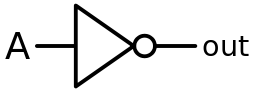
<p>You may remember these logical gate diagrams, like for the NOT gate:</p>

<p><img src="../images/multiverse-part-2/not-gate.png" alt="A logical NOT gate symbol" /></p>

<p>This logical gate transforms a single bit, 0 into a 1 or a 1 into a 0. It’s one of the basic building blocks of every CPU and computing device.</p>

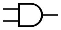
<h3 id="and-gate">AND Gate:</h3>

<p>The AND gate outputs a 1 only if both inputs are a 1.</p>

<p><img src="../images/multiverse-part-2/and-gate.png" alt="A logical AND gate symbol" /></p>

\[0 \wedge 0 = 0\]

\[0 \wedge 1 = 0\]

\[1 \wedge 1 = 1\]

<h3 id="xor-gate">XOR Gate:</h3>

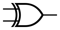
<p>The XOR (exclusive OR) gate outputs a 1 if only one of the inputs is a 1.</p>

<p><img src="../images/multiverse-part-2/xor-gate.png" alt="A logical XOR gate symbol" /></p>

\[0 \oplus 0 = 0\]

\[0 \oplus 1 = 1\]

\[1 \oplus 1 = 0\]

<h3 id="combining-gates">Combining gates</h3>

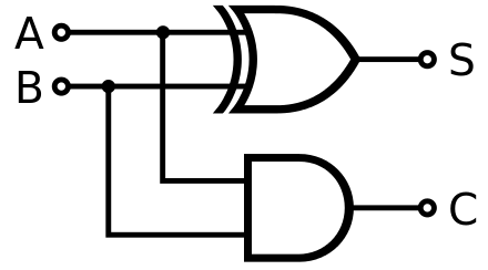
<p>We can combine the XOR and AND gates to build a very simple computer that adds bits! First, let’s see what happens when we mathematically add two binary bits:</p>

\[0 + 0 = 00\]

\[0 + 1 = 01\]

\[1 + 0 = 01\]

\[1 + 1 = 10\]

<p>Here is the logical gate diagram for an adder:</p>

<p><img src="../images/multiverse-part-2/adder-gate.png" alt="A logical XOR gate symbol" /></p>

<p>Our adder takes two inputs, A, and B, which represent each input bit. There are two output bits because adding 1 and 1 gives us a 2-bit result. For a result representing the binary value <code class="language-plaintext highlighter-rouge">01</code> C will be the first digit, <code class="language-plaintext highlighter-rouge">0</code>, and S will be the second digit, <code class="language-plaintext highlighter-rouge">1</code>. For a result of <code class="language-plaintext highlighter-rouge">10</code>, C will be <code class="language-plaintext highlighter-rouge">1</code> and S will be <code class="language-plaintext highlighter-rouge">0</code>.</p>

<p>Here are the results of running the binary adder:</p>

<table>
  <thead>
    <tr>
      <th>A</th>
      <th>B</th>
      <th>C</th>
      <th>S</th>
    </tr>
  </thead>
  <tbody>
    <tr>
      <td>0</td>
      <td>0</td>
      <td>0</td>
      <td>0</td>
    </tr>
    <tr>
      <td>0</td>
      <td>1</td>
      <td>0</td>
      <td>1</td>
    </tr>
    <tr>
      <td>1</td>
      <td>0</td>
      <td>0</td>
      <td>1</td>
    </tr>
    <tr>
      <td>1</td>
      <td>1</td>
      <td>1</td>
      <td>0</td>
    </tr>
  </tbody>
</table>

<p>Go ahead and trace the result of each gate given each combination of 0 and 1 for A and B and see what you get.</p>

<h3 id="data-flow-in-logic-gates">Data flow in logic gates</h3>

<p>In classical computers, in a sense you can say the <em>data</em> is moving around through the gates. You can think of each gate as a function that takes data input, may modify it, then output a result.</p>

<p><img src="../images/multiverse-part-2/logic-gates-vlsi.png" alt="Logical gates combined into a large component" /></p>

<p>Utlimately these logic gates form the thousands of building blocks that combine into our modern day, general purpose “integrated circuits” (e.g. CPUs).</p>

<p>A classical computer is limited in how many of these gate operations it can perform per second. For example an Intel i9 14900HX can run these gate operations up to 5,800,000,000 times per second. There is an upper limit on how many calculations a CPU can try per second to try and solve a problem.</p>

<h2 id="the-fancy-new-quantum-gates">The fancy new quantum gates</h2>

<p>You’ve seen how logic gates work in classical computers operating on bits. Starting out, it may seem that quantum and classic logic gates are similar, but we’ll see that quantum computing is a complete shift in how we think of computing.</p>

<p>Now let’s dive into some of the foundational quantum gates. For now we’re just going to focus on their behavior but just know that the way these logical gates are implemented in actual quantum coputers vary and are still under constant development and innovation.</p>

<h3 id="quantum-circuit-diagrams">Quantum circuit diagrams</h3>

<p><img src="../images/multiverse-part-2/basic-circuit-diagram.png" alt="A basic quantum circuit diagram" height="200" /></p>

<p>Here is the most basic quantum circuit diagram in the world. It does absolutely nothing, except measure the values of two qubits. Let’s break it down:</p>

<p>\(q_0\) and \(q_1\) are two qubits. By convention, they are intialized to \(\ket{0}\).</p>

<p>Whoah, wait a minute! What’s this \(\ket{0}\) thing? Well for now you can think of it just like a regular binary 0 from the classical world. \(\ket{1}\) represents a 1. It’s pronounced “ket-zero” or “ket-one.”</p>

<p>Back to the diagram, the <code class="language-plaintext highlighter-rouge">c</code> represents our “classical register.” You can think of this like the wire where our classical computer will read from to get the values of each qubit. The register has 2 outputs (shown by that <code class="language-plaintext highlighter-rouge">2</code> hovering next to the <code class="language-plaintext highlighter-rouge">c</code>), one for each qubit. So here we have qubit \(q_0\) outputting to classical register \(c_0\) and qubit \(q_1\) outputting to register \(c_1\).</p>

<p>There’s only one way to get data from a qubit - that is to “measure it.” That is what those meter icons represent. You measure a qubit and the result gets sent to the classical register. This touches on a core feature of quantum computing - the idea of superposition, measurement, and risking the life of Schrödinger’s cat - but we’ll get to that in the future.</p>

<p>So from the above diagram we’d read the values of \(c_0\) and \(c_1\) and get <code class="language-plaintext highlighter-rouge">00</code> because \(q_0\) and \(q_1\) are both initialized to \(\ket{0}\).</p>

<h3 id="swap-gate">SWAP Gate</h3>

<p><img src="../images/multiverse-part-2/quantum-swap-gate.jpg" alt="SWAP Gate" height="200" /></p>

<p>A swap gate is very simple. It simply swaps the inputs. If <code class="language-plaintext highlighter-rouge">q0</code> is \(\ket{1}\) and <code class="language-plaintext highlighter-rouge">q1</code> is \(\ket{0}\) then after the gate <code class="language-plaintext highlighter-rouge">q0</code> becomes \(\ket{0}\) and <code class="language-plaintext highlighter-rouge">q1</code> becomes \(\ket{1}\). Our classical registers would read <code class="language-plaintext highlighter-rouge">01</code> after the measurements.</p>

<p>Here’s a table to map all combinations of \(\ket{0}\) and \(\ket{1}\):</p>

<table>
  <thead>
    <tr>
      <th>\(q_0\)</th>
      <th>\(q_1\)</th>
      <th>\(c_0\)</th>
      <th>\(c_1\)</th>
    </tr>
  </thead>
  <tbody>
    <tr>
      <td>\(\ket{0}\)</td>
      <td>\(\ket{0}\)</td>
      <td>0</td>
      <td>0</td>
    </tr>
    <tr>
      <td>\(\ket{0}\)</td>
      <td>\(\ket{1}\)</td>
      <td>1</td>
      <td>0</td>
    </tr>
    <tr>
      <td>\(\ket{1}\)</td>
      <td>\(\ket{0}\)</td>
      <td>0</td>
      <td>1</td>
    </tr>
    <tr>
      <td>\(\ket{1}\)</td>
      <td>\(\ket{1}\)</td>
      <td>1</td>
      <td>1</td>
    </tr>
  </tbody>
</table>

<h3 id="cnot-gate">CNOT Gate</h3>

<p>The CNOT is similar to your familiar old NOT gate. However, it has some special behaviors that we’ll cover later. For now, just know that it has a special “control” input that tells the gate whether to actually perform the NOT operation.</p>

<p><img src="../images/multiverse-part-2/cnot.png" alt="CNOT Gate" height="200" /></p>

<p>In the example above, <code class="language-plaintext highlighter-rouge">q0</code> is set to \(\ket{1}\) and is sent to the “control” input of the gate. <code class="language-plaintext highlighter-rouge">q1</code> is set to \(\ket{0}\) and is sent to the operand input. The result is that <code class="language-plaintext highlighter-rouge">q1</code> changes to \(\ket{1}\). If <code class="language-plaintext highlighter-rouge">q0</code> were set to \(\ket{0}\) then <code class="language-plaintext highlighter-rouge">q1</code> would remain \(\ket{0}\).</p>

<h3 id="h-gate">H Gate</h3>

<p>The H Gate, also known as the Hadamard gate, does something interesting.</p>

<p><img src="../images/multiverse-part-2/h-gate.png" alt="H Gate" height="200" /></p>

<p>By default, qubit <code class="language-plaintext highlighter-rouge">q0</code> is set to \(\ket{0}\). If we were to run this circuit once, when we measure it we may get a \(\ket{0}\), but we may also randomly get a \(\ket{1}\). If you run this circuit repeatedly, about 50% of the time you get one result or the other. In a way this is like a random number generator, but behind the scenes, the H gate puts the qubit into <strong>Superposition</strong>.</p>

<p>One of the unique behaviors of quantum physics is that certain particles, for example electrons, are in an unknown state until we “measure” that thing. What do we mean by “measure?” Well that is an enormous philosophical question we don’t have time for here.</p>

<p><img src="../images/multiverse-part-2/electron.jpg" alt="Measuring an electron" height="200" /></p>

<p>But to simplify, for an electron orbiting an atomic nucleus, we don’t know the actual position of that electron until we fire a laser at it (“measure” it) and read how the field of the electron altered the course of photons emitted by the laser. But we only know the position in that moment of time. We can measure this electron multiple times and get a probability distribution of where that electron tends to be located.</p>

<p>When we measure a qubit and put the result into the classical registers, the value that is measured is not binary, but it’s converted into a 0 or 1 value. A quantum computer interprets our quantum gates as instructions on how to alter the probability of the qubit of being converted into that 1 or 0 value.</p>

<p>Let’s say we use a 6-sided die to represent a qubit. And imagine it’s constantly spinning/rolling until we measure it. You could decide that a roll of 1-3 would give you a 0 and a roll of 4-6 would give you a 1. So when we “measure” the die by letting it fall on the table and settle onto a side, we convert the number we rolled into a 0 or 1 bit.</p>

<p>So to recap, the H gate takes our qubit that has a known state, either \(\ket{0}\) or \(\ket{1}\), and puts it into an unknown state, where if measured, will give us a 50% chance of getting a \(\ket{0}\) or \(\ket{1}\).</p>

<p>And that’s it! These are the building blocks to creating all kinds of fun quantum circuits. In the next part, we’ll dig into more quantumness and some simple mathematical notation to represent qubits.</p>

<p><img src="../images/multiverse-part-2/everything.png" alt="Scenes from the movie &quot;Everything, Everywhere, All at Once&quot;" height="200" /></p>

<p>But please beware! Any time we put a qubit into superposition and measure it, we are creating two new universes, one where the qubit is 0 and the other where it is 1. So please limit this operation so that the multiverse doesn’t run out of memory 😅</p>

<p>Next article: <a href="/programming-the-multiverse-part-3/">Part 3 - Superposition and Probability</a></p>]]></content><author><name>Erica Kastner</name></author><category term="quantum_computing" /><summary type="html"><![CDATA[In part 2 we’ll go over some very simple quantum gates and explore our first concept that makes quantum computing “quantum” — Superposition.]]></summary></entry><entry><title type="html">Programming the Multiverse: Part 1 - Introduction</title><link href="https://erica.works/programming-the-multiverse-part-1/" rel="alternate" type="text/html" title="Programming the Multiverse: Part 1 - Introduction" /><published>2024-03-13T02:12:17+00:00</published><updated>2024-03-13T02:12:17+00:00</updated><id>https://erica.works/programming-the-multiverse-part-1</id><content type="html" xml:base="https://erica.works/programming-the-multiverse-part-1/"><![CDATA[<p>Welcome to <em>Programming the Multiverse</em>, a blog series introduction to quantum computing for imperative programmers!</p>

<p><em>Note: You can skip to the table of contents <a href="#table-of-contents">here</a></em></p>

<p>If you’re familiar with programming with classical languages, such as Python, Ruby, or Java, and you have seen binary logic gates (NOT, OR, AND) before, this guide is for you!</p>

<p>The goal of this series is to get you familiar with how quantum algorithms work and have some fun with some programming problems. The intention is to introduce topics gently and intuitively, rather than using lots of jargon, diving straight into Bloch Spheres, or showing off fancy equations (we’ll keep them super simple).</p>

<h2 id="what-is-quantum-computing">What is Quantum Computing?</h2>

<p>Anything that uses the term “quantum” means using some of the special physical properties of subatomic particles like entanglement, superposition, and tunneling. We’ll get into what that means later. But unlike “classical” computers (i.e. the computers you use on a daily basis), quantum computers (QC) use these weird (some would say “spooky!”) quantum behaviors to their advantage.</p>

<h2 id="classical-computers-are-boring-but-reliable">Classical computers are boring, but reliable</h2>

<p>Classical computers are great when you want to perform a scripted task quickly. They excel at CRUD operations - creating, reading, updating, and deleting data.</p>

<h2 id="quantum-computers-are-weird-but-useful">Quantum computers are weird, but useful</h2>

<p>QC has traditionally been a hammer in search of nails, but some uses are slowly emerging. AI and QC seem to be a promising match as well as optimizing logistical problems. Instead of scripting out a process in steps, QC finds optimal paths through forests of data. Whereas classical computers try to Hulk Smash their way into a building, QC tries all the possible secret entrances simultaneously. But quantum computers are also a little flakey at the moment. Today they require strategies to reduce “noise” and multiple runs to get a set of results that give you an “average” answer.</p>

<h2 id="wait-what-does-the-multiverse-have-to-do-with-this">Wait what does the Multiverse have to do with this?</h2>

<p>One explanation for how quantum mechanics operates (the <a href="https://en.wikipedia.org/wiki/Many-worlds_interpretation">“Many Worlds” interpretation</a>) states that every possible thing that can happen plays out in an infinite number of parallel universes branching out from the present. You just happen to be traveling down a certain branch of reality. With quantum computing, in a sense it’s like getting to define the possible set of multiverses that emerge from the present.</p>

<p>So prepare for a mind-bending ride!</p>

<h2 id="table-of-contents">Table of Contents</h2>

<ul>
  <li><a href="/programming-the-multiverse-part-2/">Part 2 - Some Basic Gates</a></li>
  <li><a href="/programming-the-multiverse-part-3/">Part 3 - Superposition and Probability</a></li>
  <li><a href="/programming-the-multiverse-part-4/">Part 4 - The Guts of Gates</a></li>
  <li><a href="/programming-the-multiverse-part-5/">Part 5 - Finally, Some Programming!</a></li>
  <li><a href="/programming-the-multiverse-part-6/">Part 6 - Kickbacks</a></li>
  <li><a href="/programming-the-multiverse-part-7/">Part 7 - Solving the BernVaz Oracle</a></li>
</ul>

<h2 id="sources">Sources</h2>

<p>If you’re interested in learning more on your own, I highly suggest these sources that provided a lot of inspiration and information for this series:</p>

<ul>
  <li><a href="https://www.edx.org/learn/quantum-computing/university-of-chicago-introduction-to-quantum-computing-for-everyone?index=product&amp;objectID=course-e08ab5d6-00e1-4cab-8e00-12d05299e906">Intro to Quantum Computing for Everyone</a> by the folks at EPiQ / UChicago, delivered by edX.</li>
  <li><a href="https://learning.edx.org/course/course-v1:UChicagoX+QUAN12000+2T2021/home">Intro to Quantum Computing for Everyone 2</a></li>
  <li><a href="https://github.com/Qiskit/textbook">Qiskit Textbook</a> from IBM</li>
</ul>]]></content><author><name>Erica Kastner</name></author><category term="quantum_computing" /><summary type="html"><![CDATA[Welcome to Programming the Multiverse, a blog series introduction to quantum computing for imperative programmers!]]></summary></entry><entry><title type="html">How to run docker containers in Intel/x86 mode on an M1 Mac</title><link href="https://erica.works/docker-on-mac-m1/" rel="alternate" type="text/html" title="How to run docker containers in Intel/x86 mode on an M1 Mac" /><published>2021-04-21T03:27:17+00:00</published><updated>2021-04-21T03:27:17+00:00</updated><id>https://erica.works/docker-on-mac-m1</id><content type="html" xml:base="https://erica.works/docker-on-mac-m1/"><![CDATA[<p>I’m working on a node.js/blitz.js/web project that uses pact via the pact-node
package. Unfortunately, this package isn’t compatible with Apple’s M1 (aarm64)
chip due to the standalone ruby (Intel/x86-only) that’s packaged with it.
Instead of trying to have two node installations for each platform, I decided to
try and get docker to build and run my app images using the amd64 platform. And
it works!</p>

<p>First, make sure you have the latest <a href="https://docs.docker.com/docker-for-mac/apple-silicon/">docker
desktop</a> that supports
aarm64 (M1).</p>

<p>Next, create a docker-compose.yml for your app (for now I’m setting up compose
so that I have to rebuild docker images on every code change, but you do have
the option of mounting your local source directory, though, there are
performance penalties to this).</p>

<p>You’ll need to specify that you want to build and run the image/container with
the linux/amd64 platform.</p>

<div class="language-yaml highlighter-rouge"><div class="highlight"><pre class="highlight"><code><span class="c1"># docker-compose.yml</span>

<span class="na">version</span><span class="pi">:</span> <span class="s2">"</span><span class="s">3.8"</span>
<span class="na">services</span><span class="pi">:</span>
  <span class="na">app</span><span class="pi">:</span>
    <span class="na">build</span><span class="pi">:</span>
      <span class="na">context</span><span class="pi">:</span> <span class="s">.</span>
    <span class="na">platform</span><span class="pi">:</span> <span class="s2">"</span><span class="s">linux/amd64"</span>
    <span class="c1"># ...</span>
</code></pre></div></div>

<p>The tricky part is that you can’t use docker-compose. First, it won’t use
docker buildx which has cross-platform building capabilities. Second, for some
weird reason, docker-compose 2.4 supported the <code class="language-plaintext highlighter-rouge">platform</code> setting but subsequent
versions did not.</p>

<p>You have to use the new <code class="language-plaintext highlighter-rouge">docker compose</code>
<a href="https://docs.docker.com/compose/cli-command/">command</a> and not the classic
<code class="language-plaintext highlighter-rouge">docker-compose</code>:</p>

<div class="language-bash highlighter-rouge"><div class="highlight"><pre class="highlight"><code>docker compose run app
</code></pre></div></div>

<h4 id="possible-tie-in-with-docker-buildx">Possible tie-in with docker buildx</h4>

<p>I did this on my local system but not 100% sure if it’s necessary. But it’s a
cool feature for managing build environments. Create a docker buildx builder
for your local app context:</p>

<div class="language-bash highlighter-rouge"><div class="highlight"><pre class="highlight"><code>docker buildx create <span class="nt">--platform</span> linux/amd64 <span class="nt">--name</span> my-app
docker buildx use my-app
</code></pre></div></div>

<p>Now when you run <code class="language-plaintext highlighter-rouge">docker buildx build -t my-app .</code> it will build the <code class="language-plaintext highlighter-rouge">my-app</code>
image using the platform specified in the builder you created.</p>]]></content><author><name>Erica Kastner</name></author><category term="docker" /><summary type="html"><![CDATA[I’m working on a node.js/blitz.js/web project that uses pact via the pact-node package. Unfortunately, this package isn’t compatible with Apple’s M1 (aarm64) chip due to the standalone ruby (Intel/x86-only) that’s packaged with it. Instead of trying to have two node installations for each platform, I decided to try and get docker to build and run my app images using the amd64 platform. And it works!]]></summary></entry><entry><title type="html">Notable Links: Software Development</title><link href="https://erica.works/notable-links-software-development/" rel="alternate" type="text/html" title="Notable Links: Software Development" /><published>2017-05-12T15:21:17+00:00</published><updated>2017-05-12T15:21:17+00:00</updated><id>https://erica.works/notable-links-software-development</id><content type="html" xml:base="https://erica.works/notable-links-software-development/"><![CDATA[<p>Great talk by Randy Shoup on <a href="http://www.ustream.tv/recorded/102858736">designing effective microservices</a> - very much in line with what I’ve been building out our message-oriented architecture at Faraday.</p>]]></content><author><name>Erica Kastner</name></author><category term="links" /><summary type="html"><![CDATA[Great talk by Randy Shoup on designing effective microservices - very much in line with what I’ve been building out our message-oriented architecture at Faraday.]]></summary></entry></feed>