In the last few posts I’ve been talking about various gates and some of the math behind them, but despite the title of this series there has been little actual programming. We now have enough components to make a basic quantum calculation. Let’s go!
Note: this post is part of my series, Programming the Multiverse
Prerequisites
I have to admit, I only know enough python to be dangerous. Ruby was always my go-to scripting language. But alas, because python is firmly embedded in the math/science communities with Jupyter Notebooks, it’s the default language for anything quantum related.
So first of all, you need python. I used homebrew to install pyenv to manage my python versions. I also use poetry to manage dependencies.
For this blog series I’ll be using IBM’s Qiskit library to define quantum circuits. It comes with some handy visualization features and allows you to compile and run your circuits on quantum simulators or even on actual quantum computers hosted by IBM.
If you’d like to follow along, simply clone the git repo for this blog series and follow the installation instructions in the README. The use of pyenv and poetry in that repo help ensure you have the right version of python that works with Qiskit 1.1.0.
Most of the code I’ll write will be in Jupyter notebooks. For simplicity, I like to render my notebooks in Visual Studio Code using the Jupyter extension but you’re free to run your own local jupyter server.
Our SWAP gate
Let’s code our first quantum circuit! We’ll be doing a simple swap on two qubits.
The first step is to import all the libraries we need:
from qiskit import QuantumCircuit, QuantumRegister, ClassicalRegister
The QuantumRegister represents a set of qubits. The ClassicalRegister represents those “wires” that we connect to the qubits when we perform a measurement and translate the result into binary zeros and ones that our classical (binary) computer can read.
The next step is to create those registers:
q = QuantumRegister(2, 'q')
c = ClassicalRegister(2, 'c')
The first line says “create two qubits labeled using a prefix of ‘q’.” The second line says “create two classical registers labeled using a prefix of ‘c’.”
Next, we create our quantum circuit (basically like our workspace) which includes our qubits and classical registers:
qc = QuantumCircuit(q, c)
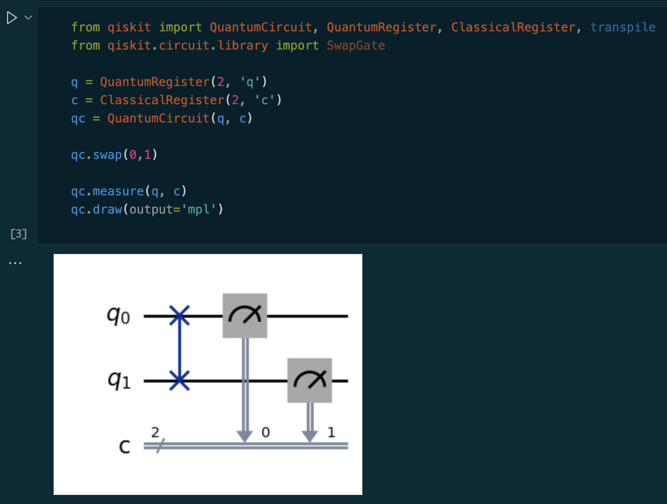
With all that boilerplate out of the way, we can start wiring up our qubits to gates. Qiskit is a bit cryptic in that you have to reference qubits by their zero-based index. So this next line says “swap qubit q0 with qubit q1”:
qc.swap(0,1)
At this point we will now measure the qubits and map the results into our classical registers:
qc.measure(q, c)
And finally, we’ll display the circuit:
qc.draw(output='mpl')
When we run this in our jupyter notebook we see this:
Qiskit can also draw your circuits using LaTeX or even ASCII art.
Another handy tool is that qiskit will show you the matrix representation of any piece of your circuit. Let’s look at the SWAP gate:
from qiskit_aer import Aer
from qiskit.visualization import array_to_latex
from IPython.display import display, Markdown

q = QuantumRegister(2, 'q')
c = ClassicalRegister(2, 'c')
qc = QuantumCircuit(q, c)

qc.swap(0,1)
# NOTE: we cannot measure if we want a unitary!

simulator = Aer.get_backend('unitary_simulator')
result = simulator.run(qc).result()
unitary = result.get_unitary(qc)
unitary.draw('latex')
The above code re-creates the circuit because we can’t use the one above that has measurements added to it. It then creates an “ideal” quantum computer simulator (we’ll explore ideal vs real quantum computers later) and runs the simulation, extracting the “unitary” matrix that represents the gate. “Unitary” is just another name for the matrix representation of our logic gates. We’ll see later that we can build single unitaries out of combinations of multiple gates.
The output gives us the expected matrix representing a basic swap:
\[\begin{bmatrix} 1 & 0 & 0 & 0 \\ 0 & 0 & 1 & 0 \\ 0 & 1 & 0 & 0 \\ 0 & 0 & 0 & 1 \\ \end{bmatrix}\]You can also output the state vector using a similar method:
simulator = Aer.get_backend('statevector_simulator')
result = simulator.run(qc).result()
state = result.get_statevector(qc)
state.draw('latex')
Which outputs the state vector representing the combined state of the two qubits:
\[\ket{00}\]Now we have all the tools we need to build all kinds of quantum circuits and evaluate their behavior using unitary matrices and state vectors.
Next article: Part 6 - Kickbacks