With superposition and phase kickback in our toolbelt, we finally have what we need to start solving some real problems.
Note: this post is part of my series, Programming the Multiverse
The Bernstein–Vazirani oracle is a toy problem that starts to show how certain problems can be solved faster with quantum computers than classical algorithms.
The BernVaz Oracle
The BernVaz oracle is like a black box that can have at least 2 inputs and an equal number of outputs. In our example we’ll have 4 inputs. The goal is to guess a secret pattern that is encoded in the oracle.
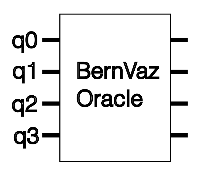
The first 3 inputs, labeled \(q_0\) through \(q_2\), are inputs where you can feed your guesses of a 0 or a 1. The outputs corresponding to each guess input do not change the value, they simply echo back your input.
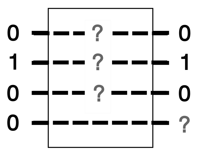
The last input, \(q_3\), is a status signal. If you correctly guess that any one of the wires is a 1, whatever value you feed into the status input will get flipped in a NOT operation. If you correctly guess a 0 on any of the inputs, \(q_3\) will not change. If you incorrectly guess a 0, \(q_3\) will also remain unchanged.
Here’s a sample for an incorrect guess:
| Inputs | Secret code | Output | |
|---|---|---|---|
| \(q_0\) | 1 | 0 | 1 |
| \(q_1\) | 0 | 1 | 0 |
| \(q_2\) | 0 | 0 | 0 |
| \(q_3\) | 1 | 1 |
Here’s a sample for correct guess:
| Inputs | Secret code | Output | |
|---|---|---|---|
| \(q_0\) | 0 | 0 | 0 |
| \(q_1\) | 1 | 1 | 1 |
| \(q_2\) | 0 | 0 | 0 |
| \(q_3\) | 1 | 0 |
A sample for a partially correct guess (note that the oracle doesn’t tell you whether you’re partially correct or totally correct):
| Inputs | Secret code | Output | |
|---|---|---|---|
| \(q_0\) | 0 | 0 | 0 |
| \(q_1\) | 1 | 1 | 1 |
| \(q_2\) | 0 | 1 | 0 |
| \(q_3\) | 1 | 0 |
And finally, a sample where we fully guess a code containing multiple ones:
| Inputs | Secret code | Output | |
|---|---|---|---|
| \(q_0\) | 0 | 0 | 0 |
| \(q_1\) | 1 | 1 | 1 |
| \(q_2\) | 1 | 1 | 1 |
| \(q_3\) | 1 | 1 |
Note that in the above example that the status input, \(q_3\) gets flipped twice.
How we would implement such an oracle
How would we implement this oracle? You may have already guessed that this involves some CNOTs. Basically we implement this by CNOTing every guess input with the status input when the secret value for the input is a 1. Here’s an example for an encoded value of \(011\):
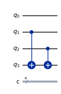
The code for this is here.
The hulk-smash way of solving the oracle
A classical computer is limited to solving this the “hulk smash” way - that is, a brute force approach. Just like if the Hulk were to break into a building by smashing down a wall.
 Image credit: serbiandude via Deviantart
We would have to guess a 1 for each input, one by one, to get an answer.
First guess:
| Inputs | Secret code | Output | |
|---|---|---|---|
| \(q_0\) | 1 | 0 | 1 |
| \(q_1\) | 0 | 1 | 0 |
| \(q_2\) | 0 | 1 | 0 |
| \(q_3\) | 1 | 1 |
This tells us that the first number is a 0 because our status input did not get flipped.
Second guess:
| Inputs | Secret code | Output | |
|---|---|---|---|
| \(q_0\) | 0 | 0 | 0 |
| \(q_1\) | 1 | 1 | 1 |
| \(q_2\) | 0 | 1 | 0 |
| \(q_3\) | 1 | 0 |
This tells us that the second number is a 1 because our status input did get flipped.
Third guess:
| Inputs | Secret code | Output | |
|---|---|---|---|
| \(q_0\) | 0 | 0 | 0 |
| \(q_1\) | 0 | 1 | 0 |
| \(q_2\) | 1 | 1 | 1 |
| \(q_3\) | 1 | 0 |
Similarly, this tells us that the third number is a 1 because our status input got flipped.
You can see that for larger oracles, we need more and more guesses. In fact, it’s a \(O(n)\) solution (for those familiar with big-Oh notation). In other words, the time taken to solve this increases at a linear rate with the increase in length of the secret code.
If this secret code was used as a password for a system, you could chose a password that’s 3 trillion bits long, which would take the world’s currently most powerful supercomputer a year to crack doing 1,700 petaflops per second.
The quantum ninja way of solving the oracle
Our new quantum computer, however, is like a ninja who is everywhere all at once and can sneak its way into any building.

Since we know how any oracle can be constructed using CNOTs, we can devise a special quantum algorithm to solve any BernVaz oracle:
- Each input is a qubit in superposition
- The status qubit is initialized to \(\ket{1}\) before putting it into superposition
- We use the H gate again on the outputs to bring every qubit back out of superposition
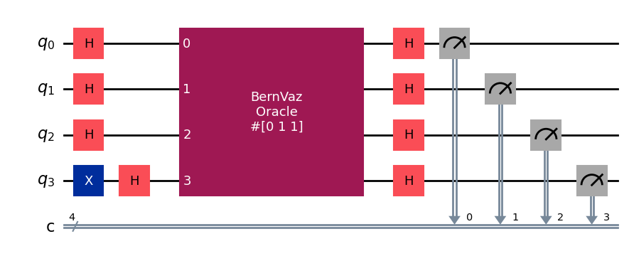
The python code to construct this circuit is here.
For this exercise, we’ll use a feature of Qiskit to build our own custom quantum gate that represents the BernVaz oracle. We define a function that returns a randomly-generated secret code along with the gate itself.
def create_random_oracle():
  # generate a 3-item array of random zeros and ones
  secret_code = random.randint(2, size=3)

  bv_circuit = QuantumCircuit(4, name="BernVaz\nOracle\n#{}".format(secret_code))

  # loop through each digit of our secret code and CNOT the appropriate
  # code qubit with the status qubit
  idx = 0
  for idx, digit in enumerate(secret_code):
    if digit == 1:
      bv_circuit.cx(idx, 3)

  # create our custom gate
  bern_vaz_oracle = bv_circuit.to_instruction()

  return [secret_code, bern_vaz_oracle]
We can then plug the oracle into our larger circuit
q = QuantumRegister(4, 'q')
c = ClassicalRegister(4, 'c')
qc = QuantumCircuit(q, c)

# put our input qubits into superposition
qc.h(0)
qc.h(1)
qc.h(2)

qc.x(3) # initialize the status qubit to |1>
qc.h(3)

secret_code, oracle = create_random_oracle()

# hook the custom gate into qubits 0-3
qc.append(oracle, [0,1,2,3])

# take the outputs out of superposition
qc.h(0)
qc.h(1)
qc.h(2)
qc.h(3)

qc.measure(0, 0)
qc.measure(1, 1)
qc.measure(2, 2)
qc.measure(3, 3)
Next we run the whole circuit through the Qasm simulator, which simulates an “ideal” quantum computer.
simulator = Aer.get_backend('qasm_simulator')
result = simulator.run(transpile(qc.reverse_bits(), simulator)).result()
This gives us the following output:
{'0111': 1024}
When we run the simulator, the simulator returns a python dictionary where each key represents a string of classical bits we got when we measured each qubit. The value associated with the key is the number of runs that resulted in that string. This is because the computer runs the simulation 1,024 times by default (more on this another time).
So yeah, our quantum computer just instantly solved the oracle!!
So how did this work?
Because we knew this oracle was implemented using CNOTs, we knew that we could use phase kickback to get the answer.
When a qubit maps to a \(\ket{0}\) value, it does not go through a CNOT. Therefore, the qubit is untouched by any other qubit. It effectively travels through two H gates:
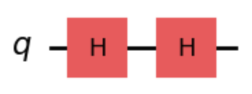
The qubit, initialized to \(\ket{0}\) returns to the \(\ket{0}\) state.
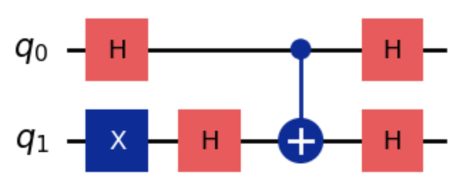
When a qubit maps to a \(\ket{1}\), this qubit is used as a control on the CNOT. The target is initialized to \(\ket{1}\) and put into superposition. Let’s look at the matrix math happening just for a single code qubit and the status qubit, which is a simple CNOT:
Our matrix multiplication for this circuit is:
\[\Psi = \overbrace{ \begin{bmatrix} \frac{1}{2} & \frac{1}{2} & \frac{1}{2} & \frac{1}{2} \\ \frac{1}{2} &-\frac{1}{2} & \frac{1}{2} &-\frac{1}{2} \\ \frac{1}{2} & \frac{1}{2} &-\frac{1}{2} &-\frac{1}{2} \\ \frac{1}{2} &-\frac{1}{2} &-\frac{1}{2} & \frac{1}{2} \\ \end{bmatrix} }^{H \otimes H} \cdot \overbrace{ \begin{bmatrix} 1 & 0 & 0 & 0 \\ 0 & 1 & 0 & 0 \\ 0 & 0 & 0 & 1 \\ 0 & 0 & 1 & 0 \\ \end{bmatrix} }^{\text{CNOT}} \cdot \overbrace{ \begin{bmatrix} 1 & 0 & 0 & 0 \\ 0 & 1 & 0 & 0 \\ 0 & 0 & 0 & 1 \\ 0 & 0 & 1 & 0 \\ \end{bmatrix} }^{I \otimes H} \cdot \overbrace{ \begin{bmatrix} 0 & \frac{\sqrt{2}}{2} & 0 & \frac{\sqrt{2}}{2} \\ \frac{\sqrt{2}}{2} & 0 & \frac{\sqrt{2}}{2} & 0 \\ 0 & \frac{\sqrt{2}}{2} & 0 & -\frac{\sqrt{2}}{2} \\ \frac{\sqrt{2}}{2} & 0 & -\frac{\sqrt{2}}{2} & 0 \\ \end{bmatrix} }^{H \otimes X} \cdot \overbrace{ \begin{bmatrix} 1 \\ 0 \\ 0 \\ 0 \end{bmatrix} }^{q_0 \otimes q_1}\]The state vector going into the CNOT is:
\[\Psi = \overbrace{ \begin{bmatrix} \frac{1}{2} & \frac{1}{2} & \frac{1}{2} & \frac{1}{2} \\ \frac{1}{2} &-\frac{1}{2} & \frac{1}{2} &-\frac{1}{2} \\ \frac{1}{2} & \frac{1}{2} &-\frac{1}{2} &-\frac{1}{2} \\ \frac{1}{2} &-\frac{1}{2} &-\frac{1}{2} & \frac{1}{2} \\ \end{bmatrix} }^{H \otimes H} \cdot \overbrace{ \begin{bmatrix} 1 & 0 & 0 & 0 \\ 0 & 1 & 0 & 0 \\ 0 & 0 & 0 & 1 \\ 0 & 0 & 1 & 0 \\ \end{bmatrix} }^{\text{CNOT}} \cdot \overbrace{ \begin{bmatrix} \frac{1}{2} \\ -\frac{1}{2} \\ \frac{1}{2} \\ -\frac{1}{2} \end{bmatrix} }^{q_0 \otimes q_1}\]This means we have a 25% chance of each combination of qubits but that the phase is negative whenever \(q_1 = \ket{1}\).
After the CNOT, the state vector becomes:
\[\Psi = \overbrace{ \begin{bmatrix} \frac{1}{2} & \frac{1}{2} & \frac{1}{2} & \frac{1}{2} \\ \frac{1}{2} &-\frac{1}{2} & \frac{1}{2} &-\frac{1}{2} \\ \frac{1}{2} & \frac{1}{2} &-\frac{1}{2} &-\frac{1}{2} \\ \frac{1}{2} &-\frac{1}{2} &-\frac{1}{2} & \frac{1}{2} \\ \end{bmatrix} }^{H \otimes H} \cdot \overbrace{ \begin{bmatrix} \frac{1}{2} \\ -\frac{1}{2} \\ -\frac{1}{2} \\ \frac{1}{2} \end{bmatrix} }^{q_0 \otimes q_1}\]The CNOT kicked the negative phase back up to the control qubit.
The key here is that when the negative phase is kicked back to \(q_0\), its individual state is \(q_0 = \frac{1}{\sqrt{2}}\ket{0} - \frac{1}{\sqrt{2}}\ket{1}\). This means when we apply the H gate to it, we have the following:
\[\overbrace{ \begin{bmatrix} \frac{1}{\sqrt{2}} & \frac{1}{\sqrt{2}} \\ \frac{1}{\sqrt{2}} & -\frac{1}{\sqrt{2}} \end{bmatrix} }^{H} \cdot \overbrace{ \begin{bmatrix} \frac{1}{\sqrt{2}} \\ -\frac{1}{\sqrt{2}} \end{bmatrix} }^{q_0} = \begin{bmatrix} (\frac{1}{\sqrt{2}} \times \frac{1}{\sqrt{2}}) + \textcolor{red}{(\frac{1}{\sqrt{2}} \times -\frac{1}{\sqrt{2}})} \\ (\frac{1}{\sqrt{2}} \times \frac{1}{\sqrt{2}}) + \textcolor{red}{(-\frac{1}{\sqrt{2}} \times -\frac{1}{\sqrt{2}})} \end{bmatrix} = \begin{bmatrix} \frac{1}{2} - \frac{1}{2} \\ \frac{1}{2} + \frac{1}{2} \end{bmatrix} = \begin{bmatrix} 0 \\ 1 \end{bmatrix}\]The negative phase of \(q_0\) caused the H gate to behave in an interesting way - it turns a qubit in superposition with negative phase into a \(\ket{1}\). We’ll cover what’s going on behind the scenes later but for now we were able to “hack” our H gate to help us!