In part 2 we’ll go over some very simple quantum gates and explore our first concept that makes quantum computing “quantum” — Superposition.
Note: this post is part of my series, Programming the Multiverse
We’re going to start with some basics. I mean, suuuuper basic. But it’s an important first step. Currently there are no widely-used programming languages for programming quantum computers the same way we write code for today’s computers. The languages that do exist are very esoteric. Instead, quantum computers today are programmed using gates similar to the logic gates we use in today’s computers. So, it’s all very low level.
So before we go into quantum gates and qubits, let’s review logic gates from the classic world.
Ye olde logick gates
You may remember these logical gate diagrams, like for the NOT gate:
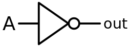
This logical gate transforms a single bit, 0 into a 1 or a 1 into a 0. It’s one of the basic building blocks of every CPU and computing device.
AND Gate:
The AND gate outputs a 1 only if both inputs are a 1.

XOR Gate:
The XOR (exclusive OR) gate outputs a 1 if only one of the inputs is a 1.

Combining gates
We can combine the XOR and AND gates to build a very simple computer that adds bits! First, let’s see what happens when we mathematically add two binary bits:
\[0 + 0 = 00\] \[0 + 1 = 01\] \[1 + 0 = 01\] \[1 + 1 = 10\]Here is the logical gate diagram for an adder:

Our adder takes two inputs, A, and B, which represent each input bit. There are two output bits because adding 1 and 1 gives us a 2-bit result. For a result representing the binary value 01 C will be the first digit, 0, and S will be the second digit, 1. For a result of 10, C will be 1 and S will be 0.
Here are the results of running the binary adder:
| A | B | C | S |
|---|---|---|---|
| 0 | 0 | 0 | 0 |
| 0 | 1 | 0 | 1 |
| 1 | 0 | 0 | 1 |
| 1 | 1 | 1 | 0 |
Go ahead and trace the result of each gate given each combination of 0 and 1 for A and B and see what you get.
Data flow in logic gates
In classical computers, in a sense you can say the data is moving around through the gates. You can think of each gate as a function that takes data input, may modify it, then output a result.

Utlimately these logic gates form the thousands of building blocks that combine into our modern day, general purpose “integrated circuits” (e.g. CPUs).
A classical computer is limited in how many of these gate operations it can perform per second. For example an Intel i9 14900HX can run these gate operations up to 5,800,000,000 times per second. There is an upper limit on how many calculations a CPU can try per second to try and solve a problem.
The fancy new quantum gates
You’ve seen how logic gates work in classical computers operating on bits. Starting out, it may seem that quantum and classic logic gates are similar, but we’ll see that quantum computing is a complete shift in how we think of computing.
Now let’s dive into some of the foundational quantum gates. For now we’re just going to focus on their behavior but just know that the way these logical gates are implemented in actual quantum coputers vary and are still under constant development and innovation.
Quantum circuit diagrams
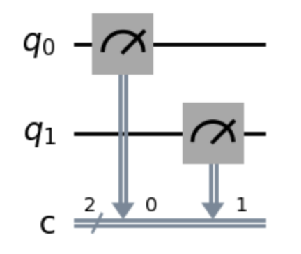
Here is the most basic quantum circuit diagram in the world. It does absolutely nothing, except measure the values of two qubits. Let’s break it down:
\(q_0\) and \(q_1\) are two qubits. By convention, they are intialized to \(\ket{0}\).
Whoah, wait a minute! What’s this \(\ket{0}\) thing? Well for now you can think of it just like a regular binary 0 from the classical world. \(\ket{1}\) represents a 1. It’s pronounced “ket-zero” or “ket-one.”
Back to the diagram, the c represents our “classical register.” You can think of this like the wire where our classical computer will read from to get the values of each qubit. The register has 2 outputs (shown by that 2 hovering next to the c), one for each qubit. So here we have qubit \(q_0\) outputting to classical register \(c_0\) and qubit \(q_1\) outputting to register \(c_1\).
There’s only one way to get data from a qubit - that is to “measure it.” That is what those meter icons represent. You measure a qubit and the result gets sent to the classical register. This touches on a core feature of quantum computing - the idea of superposition, measurement, and risking the life of Schrödinger’s cat - but we’ll get to that in the future.
So from the above diagram we’d read the values of \(c_0\) and \(c_1\) and get 00 because \(q_0\) and \(q_1\) are both initialized to \(\ket{0}\).
SWAP Gate
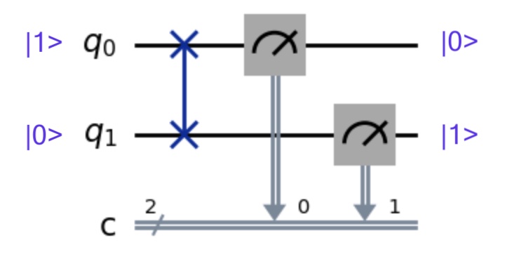
A swap gate is very simple. It simply swaps the inputs. If q0 is \(\ket{1}\) and q1 is \(\ket{0}\) then after the gate q0 becomes \(\ket{0}\) and q1 becomes \(\ket{1}\). Our classical registers would read 01 after the measurements.
Here’s a table to map all combinations of \(\ket{0}\) and \(\ket{1}\):
| \(q_0\) | \(q_1\) | \(c_0\) | \(c_1\) |
|---|---|---|---|
| \(\ket{0}\) | \(\ket{0}\) | 0 | 0 |
| \(\ket{0}\) | \(\ket{1}\) | 1 | 0 |
| \(\ket{1}\) | \(\ket{0}\) | 0 | 1 |
| \(\ket{1}\) | \(\ket{1}\) | 1 | 1 |
CNOT Gate
The CNOT is similar to your familiar old NOT gate. However, it has some special behaviors that we’ll cover later. For now, just know that it has a special “control” input that tells the gate whether to actually perform the NOT operation.
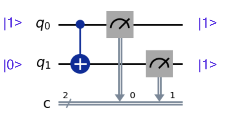
In the example above, q0 is set to \(\ket{1}\) and is sent to the “control” input of the gate. q1 is set to \(\ket{0}\) and is sent to the operand input. The result is that q1 changes to \(\ket{1}\). If q0 were set to \(\ket{0}\) then q1 would remain \(\ket{0}\).
H Gate
The H Gate, also known as the Hadamard gate, does something interesting.
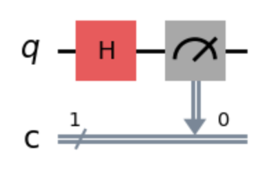
By default, qubit q0 is set to \(\ket{0}\). If we were to run this circuit once, when we measure it we may get a \(\ket{0}\), but we may also randomly get a \(\ket{1}\). If you run this circuit repeatedly, about 50% of the time you get one result or the other. In a way this is like a random number generator, but behind the scenes, the H gate puts the qubit into Superposition.
One of the unique behaviors of quantum physics is that certain particles, for example electrons, are in an unknown state until we “measure” that thing. What do we mean by “measure?” Well that is an enormous philosophical question we don’t have time for here.
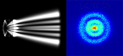
But to simplify, for an electron orbiting an atomic nucleus, we don’t know the actual position of that electron until we fire a laser at it (“measure” it) and read how the field of the electron altered the course of photons emitted by the laser. But we only know the position in that moment of time. We can measure this electron multiple times and get a probability distribution of where that electron tends to be located.
When we measure a qubit and put the result into the classical registers, the value that is measured is not binary, but it’s converted into a 0 or 1 value. A quantum computer interprets our quantum gates as instructions on how to alter the probability of the qubit of being converted into that 1 or 0 value.
Let’s say we use a 6-sided die to represent a qubit. And imagine it’s constantly spinning/rolling until we measure it. You could decide that a roll of 1-3 would give you a 0 and a roll of 4-6 would give you a 1. So when we “measure” the die by letting it fall on the table and settle onto a side, we convert the number we rolled into a 0 or 1 bit.
So to recap, the H gate takes our qubit that has a known state, either \(\ket{0}\) or \(\ket{1}\), and puts it into an unknown state, where if measured, will give us a 50% chance of getting a \(\ket{0}\) or \(\ket{1}\).
And that’s it! These are the building blocks to creating all kinds of fun quantum circuits. In the next part, we’ll dig into more quantumness and some simple mathematical notation to represent qubits.

But please beware! Any time we put a qubit into superposition and measure it, we are creating two new universes, one where the qubit is 0 and the other where it is 1. So please limit this operation so that the multiverse doesn’t run out of memory 😅
Next article: Part 3 - Superposition and Probability