In part 4 we’re going to go over the logical internals of some of these gates to see how each gate manupilates a qubit’s probability of being a 0 or 1.
Note: this post is part of my series, Programming the Multiverse
As we saw in Part 3, a qubit has a formula associated with it, called bra-ket notation, that describes its probability of being a 0 or 1:
\[\ket{\psi} = a\ket{0} + b\ket{1}\]When we apply gates to the qubits, we’re adjusting a and b and the squares of a and b have to add up to a 100% probability (or just 1 in math terms):
\[\vert{a}\vert^{2} + \vert{b}\vert^{2} = 1\]So how do we get at those a’s and b’s?
The magic matrices
Let’s take a look at a simple gate, the Pauli-X gate.
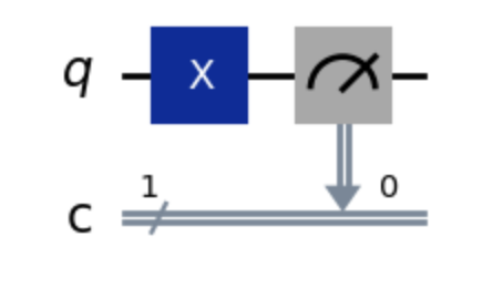
This is essentially a NOT operation on a qubit (it’s a simpler version of our earlier CNOT, but without the control input). You give it a \(\ket{0}\) and get a \(\ket{1}\) and vice-versa.
If we dig inside the Pauli-X we discover that it’s hiding a magic matrix!
\[\left[ \begin{array}{cc} 0 & 1 \\ 1 & 0 \end{array} \right]\]What’s a matrix? If you never took linear algebra or have repressed those memories, a matrix is like a two-dimensional array that has m rows and n columns.
The cool thing about matrices is that you can do math on them. When we apply a Pauli-X gate to a qubit, we are doing some matrix multiplication.
But first, in order to do this matrix multiplication, we have to turn our qubit into a matrix.
So let’s take our \(\ket{0}\) qubit, which is represented by:
\[1\ket{0} + 0\ket{1}\]We can take those a and b terms and put them into a 2-row by 1-column matrix (also called a unit vector):
\[\left[ \begin{array}{c} a \\ b \end{array} \right]\]So placing our 1 and 0, we get:
\[\left[ \begin{array}{c} 1 \\ 0 \end{array} \right]\]Now we can do the matrix multiplication (also known as the dot product). We always place the qubit matrix on the right and the gate matrix on the left:
\[A \cdot B = \left[ \begin{array}{cc} 0 & 1 \\ 1 & 0 \end{array} \right] \cdot \left[ \begin{array}{c} 1 \\ 0 \end{array} \right]\]When we multiply, we take every row in the left-hand matrix, A and multiply it by each column in the right-hand matrix. Let’s start with row 1 and column 1, the result of which we’ll put into the top cell of a new 2x1 matrix:
\[A \cdot B = \left[ \begin{array}{cc} \textcolor{red}{0} & \textcolor{red}{1} \\ 1 & 0 \end{array} \right] \cdot \left[ \begin{array}{c} \textcolor{red}{1} \\ \textcolor{red}{0} \end{array} \right] = \left[ \begin{array}{c} \textcolor{red}{?} \\ ? \end{array} \right]\]Remember, our rows are labeled \(m\) and our columns are \(n\). To designate a cell, we’ll refer to a row and column from \(A\) as \(A_{mn}\). Our new 2x1 matrix we’ll call \(C\).
\[A \cdot B = \left[ \begin{array}{cc} \textcolor{red}{A_{1,1}} & \textcolor{red}{A_{1,2}} \\ A_{2,1} & A_{2,2} \end{array} \right] \cdot \left[ \begin{array}{c} \textcolor{red}{B_{1,1}} \\ \textcolor{red}{B_{2,1}} \end{array} \right] = \left[ \begin{array}{c} \textcolor{red}{C_{1,1}} \\ C_{2,1} \end{array} \right]\]To get the first cell in \(C\), we loop through each position in the row/column and multiply each cell in \(A\) with the matching cell in \(B\), then add them up:
\[C_{1,1} = (A_{1,1} \times B_{1,1}) + (A_{1,2} \times B_{2,1})\]To get the second cell in \(C\) we operate on row 2 of the gate matrix:
\[C_{2,1} = (A_{2,1} \times B_{1,1}) + (A_{2,2} \times B_{2,1})\]If you, like me, get sick of doing matrix multiplication by hand, you can use one of many online tools or use a programming language like Ruby or Python that have great matrix support.
OK, so when we multiply our input matrix by the gate matrix, we get:
\[\left[ \begin{array}{cc} 0 & 1 \\ 1 & 0 \end{array} \right] \cdot \left[ \begin{array}{c} 1 \\ 0 \end{array} \right] = \left[ \begin{array}{c} 0 \\ 1 \end{array} \right]\]And we transform the resulting matrix back into bra-ket notation by putting \(C_{1,1}\) into a and \(C_{2,1}\) into b:
\[0\ket{0} + 1\ket{1} = \ket{1}\]We’ve done it! We flipped the qubit!
More inputs, bigger matrices
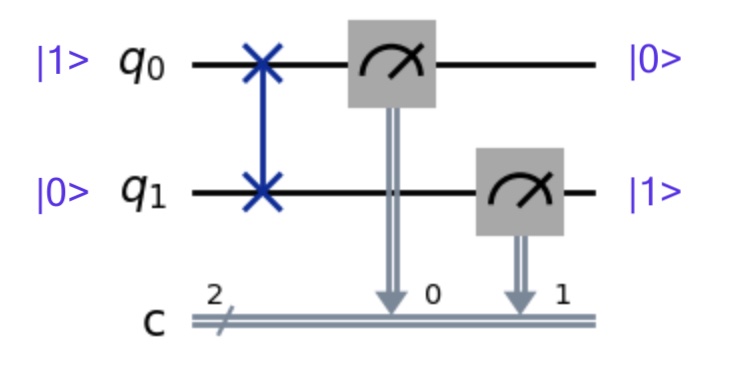
We just did the math for a quantum gate operating on a single qubit using a dot product. But let’s see what happens with a gate operating on two qubits. Let’s work with the SWAP:
The SWAP gate is represented by this magic matrix:
\[\left[ \begin{array}{cccc} 1 & 0 & 0 & 0 \\ 0 & 0 & 1 & 0 \\ 0 & 1 & 0 & 0 \\ 0 & 0 & 0 & 1 \end{array} \right]\]We need to do a dot product against our qubit vectors, but they’re too small to work with that matrix built for two inputs. We need a bigger vector!
A global representation of our qubit state
Earlier, we converted our qubit’s Dirac notation representation of \(q_0 = a\ket{0} + b\ket{1}\) into a vector that looks like:
\[q_0 = \left[ \begin{array}{c} a \\ b \end{array} \right]\]And we can do the same with qubit \(q_1\):
\[q_{1} = c\ket{0} + d\ket{1} = \left[ \begin{array}{c} c \\ d \end{array} \right]\]What we want now is a vector representing the probabilities of getting every combination of each qubit’s possible values:
\[q_{0} \otimes q_{1} = ac\ket{00} + ad\ket{01} + bc\ket{10} + bd\ket{11}\]We some alchemy at our disposal, an arcane tool called a tensor product (more specifically, a Kronecker product) we can perform on the two vector matrices. Now you can sound fancy at your next cocktail party and talk about tensors.

How to do a tensor product
For two matrices A and B, where the dimensions of A are \(m \times n\) and the dimensions of B are \(p \times q\), we get a new matrix C that has dimensions \(pm \times qn\).
When we do a tensor product of our qubits, we essentially create a grid with all the possible combinations of each element of A and each element of B:
So plugging our numbers in for our two qubits, let’s set \(q_0\) to \(\ket{1}\) and \(q_1\) to \(\ket{0}\):
\[q_{0} = 0\ket{0} + 1\ket{1}\] \[q_{1} = 1\ket{0} + 0\ket{1}\] \[q{0} \otimes q{1} = \left[ \begin{array}{c} 0 \\ 1 \end{array} \right] \otimes \left[ \begin{array}{c} 1 \\ 0 \end{array} \right] = \left[ \begin{array}{c} 0 \times 1 \\ 0 \times 0 \\ 1 \times 1 \\ 1 \times 0 \end{array} \right] = \left[ \begin{array}{c} 0 \\ 0 \\ 1 \\ 0 \end{array} \right]\]Finally, converting that vector back into our Dirac notation, we have:
\[q_{0} \otimes q_{1} = 0\ket{00} + 0\ket{01} + 1\ket{10} + 0\ket{11}\]We have a 100% chance of getting a combined state of \(\ket{10}\). In other words, \(q_0=\ket{1}\) and \(q_1 = \ket{0}\)
You can view the python code for this operation here.
Performing the swap
Now we can do a regular dot product between the magic matrix that represents a SWAP gate and the vector representing the combined state of our qubits. Note that the initial state vector is always on the right-hand side. When we do the multiplication we get a new output vector that represents the combined states of our qubits after the fact.
\[\left[ \begin{array}{cccc} 1 & 0 & 0 & 0 \\ 0 & 0 & 1 & 0 \\ 0 & 1 & 0 & 0 \\ 0 & 0 & 0 & 1 \end{array} \right] \left[ \begin{array}{c} 0 \\ 0 \\ 1 \\ 0 \end{array} \right] = \left[ \begin{array}{c} 0 \\ 1 \\ 0 \\ 0 \end{array} \right]\]Which we put back into our super tensor ultra qubit:
\[0\ket{00} + 1\ket{01} + 0\ket{10} + 0\ket{11}\]This means we have a 100% chance of a combination of 0 and 1, Which means our two qubits are:
\[q_0 = \ket{0}\] \[q_1 = \ket{1}\]And that’s the magic behind a Freaky Qubit Friday!
OK that’s enough math for now, and trust me, you won’t normally need to do any matrix multiplication by hand unless you need to deeply debug something. But it’s good to know why everything is happening. But eventually you’ll be able to just glance at a matrix and see some patterns, like identity matrices, that give you an idea of what’s going to happen when you apply it.
Next article: Part 5 - Finally, Some Programming!